Posted on February 3, 2026February 3, 2026 in farms, insects, plants

Mapping Flowers, Watching Bugs, & Building Habitat.

By Claudia & Conrad.

INTRODUCTION: Basic Premises.

It is perhaps useful to start from a few basic facts:

While certainly not necessary for all crop production, many crops require pollinators for the production of the crop itself and/or the seeds of that crop and/or are assisted by the biocontrol provided by the aphid-feeding larvae of wasps and hover flies who, as adults, feed on nectar.
With roughly 450 species of bees known from New York, plus numerous other flower visitors including many wasps, hoverflies and various butterflies and moths, flower visitors form an appreciable part of our insect biodiversity.
The relationships amongst various flower visitors and various flowers illustrates the maxim, “different strokes for different folks”. In other words, the flower preferences of different bees (not to mention other insects) can vary markedly amongst species, reflecting varying needs and offerings (including the fit of flower and insect morphological traits, coincidence of flight and flowering seasons, and the satisfaction of intricate insect nutritional requirements), co-evolutionary histories, and coincidental preferences.
Our own species has clear aesthetic flower preferences, which regularly do not align with those of all flower visitors.
The flower offering of a given farm is composed of several groups of flowers: those flowers intentionally planted for cut flowers and/or insect habitat, the flowers of crop plants where fruits are the main crop (e.g., tree fruits and berries, but also tomatoes, peppers, eggplants, squash, cucumbers, etc.), the flowers of crops (including cover crops) wherein the flowers are of little importance to production, and true wild flowers (sometimes considered weeds) composed of those native and non-native flowers that grow on farms in cultivated beds, as low blooms in cut drive strips, or as wild growth in edges, fallows and other nearby lightly-managed habitats.
By and large, human attention tends to focus on the intentionally grown flowers, with little notice paid to the potential ecological value of wild-growing flowers, except where they are considered weeds.
Finally, as a result of all of the above, a farm’s pollinator and biocontrol community and its overall insect biodiversity are shaped by a variety of intentional and unintentional flower management actions, often based on economic or aesthetic criteria and sometimes only partially informed by ecological considerations.

Starting from these premises, our work during the summer of 2025 sought to better understand the distribution and insect use of flowers on nine different farms in the Mid-Hudson Valley. Which species of flowers occurred on these farms during the growing season? Were they native or non-native? Were they wild-growing or cultivated? Where did they occur on the farm? Which insects used each of the different flowers? And, ultimately, how might a farm’s flower management be tweaked to enhance the community of flower-visiting insects?

WORDS OF CAUTION: We’re Hardly Perfect.

Several words of caution regarding the short-comings of our work are appropriate.

First, while we focused on summer flowers (June-mid Sept.) within our study areas as a key resource for flower-visiting insects, mid-season flower-availability is definitely not the only factor affecting their success. Other influences include the degree of freedom from conventional or organic pesticide exposure (see here for Xerces summary of the impacts of organic pesticides), availability of overwintering and brood sites (and, in the case of parasitoids, of larval hosts), the availability of flowers during the “shoulder seasons” (when we didn’t do surveys), competition and predation by other co-occurring animals, and flower availability outside of our study areas.

Second, we only looked at nine farms and made only three visits to each. Flower preferences may well vary in relation to flower maturity, time of day, weather, and the life-history stage of the insects. Also, each farm is different and if one wants to extract generalities, then the more farms the better. These are intricacies our observations did not address. Practicality more than optimal study design dictated the number of farms and outings.

Lastly, practicality also determined what we could do during each outing. The scale and nature of our study was limited by the self-imposed restriction of not spending more than a half day at each farm. This meant that we only mapped flowers on a portion of each farm and used quick and relatively subjective flower abundance estimates. Perhaps most importantly, it meant that we were satisfied with relatively crude taxonomic identification of the various flower visitors. While it was possible to identify the species of several flower visitors on the wing during surveys and to name several more from photographs, we did not undertake the specimen collection that would have permitted more precise identification of most insects observed. Instead, we field-identified most flower-visiting insects only to general groups, such as bumble bees, hover flies, wasps, etc. (see below for all taxonomic categories used).

All these cautions mean that, at best, our flower favorability maps show the potential for a given patch to support a particular group of insects from the perspective of floral offering. If we compare our predicted flower favorability ratings for an entire farm with the observed rates of flower visitors at that farm on that date, the relationship is scant. The best that can be said is that farms with substantially below average flower offerings do seem to have somewhat lower visitation rates than those with more favorable flowers, but that boost seems to peak pretty quickly. This implies that either our higher assessments are too rough or that once flower visitors have the minimum flower offering that they need, then other factors such as nest sites become limiting and so more flowers don’t boost populations.

In sum, if you read any of this and think, “Geesum, this study would have been better if they had ….”, then you’re probably right. Please do share such thoughts however, maybe we can do better the second time around!

METHODS: What We Did.

What did we do? We worked in parallel with Claudia surveying the flowers and Conrad observing the flower visitors.

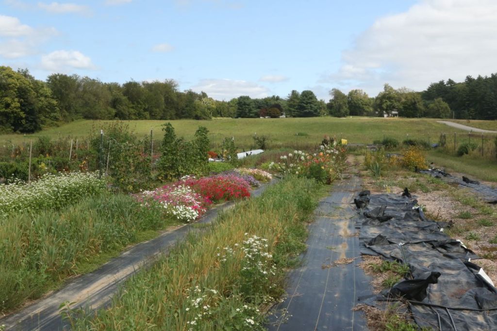
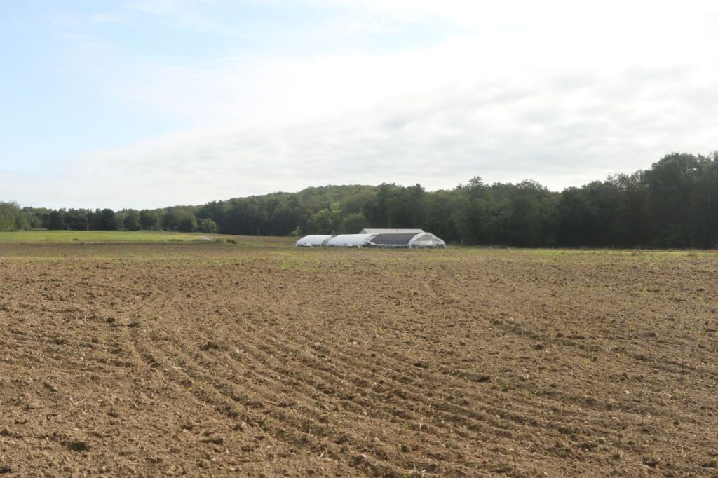
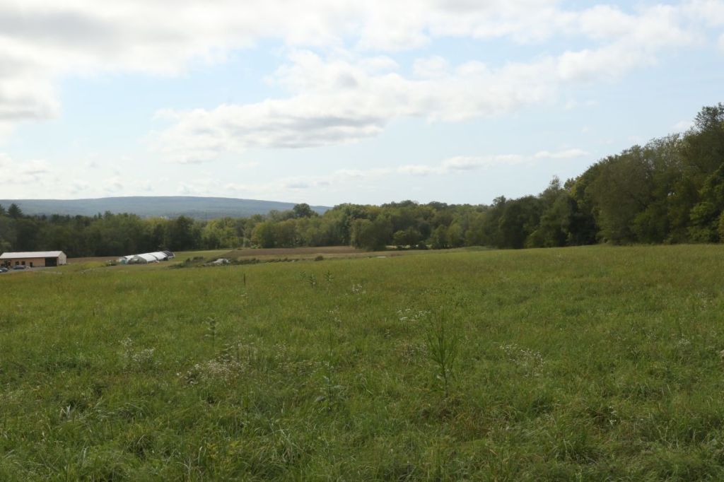
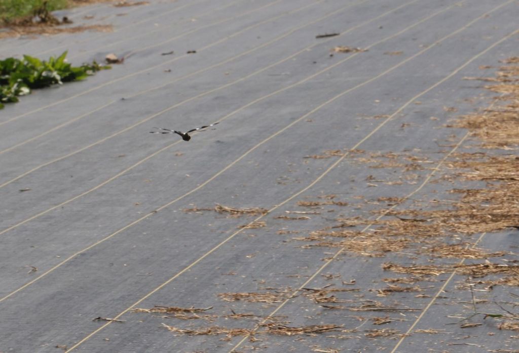
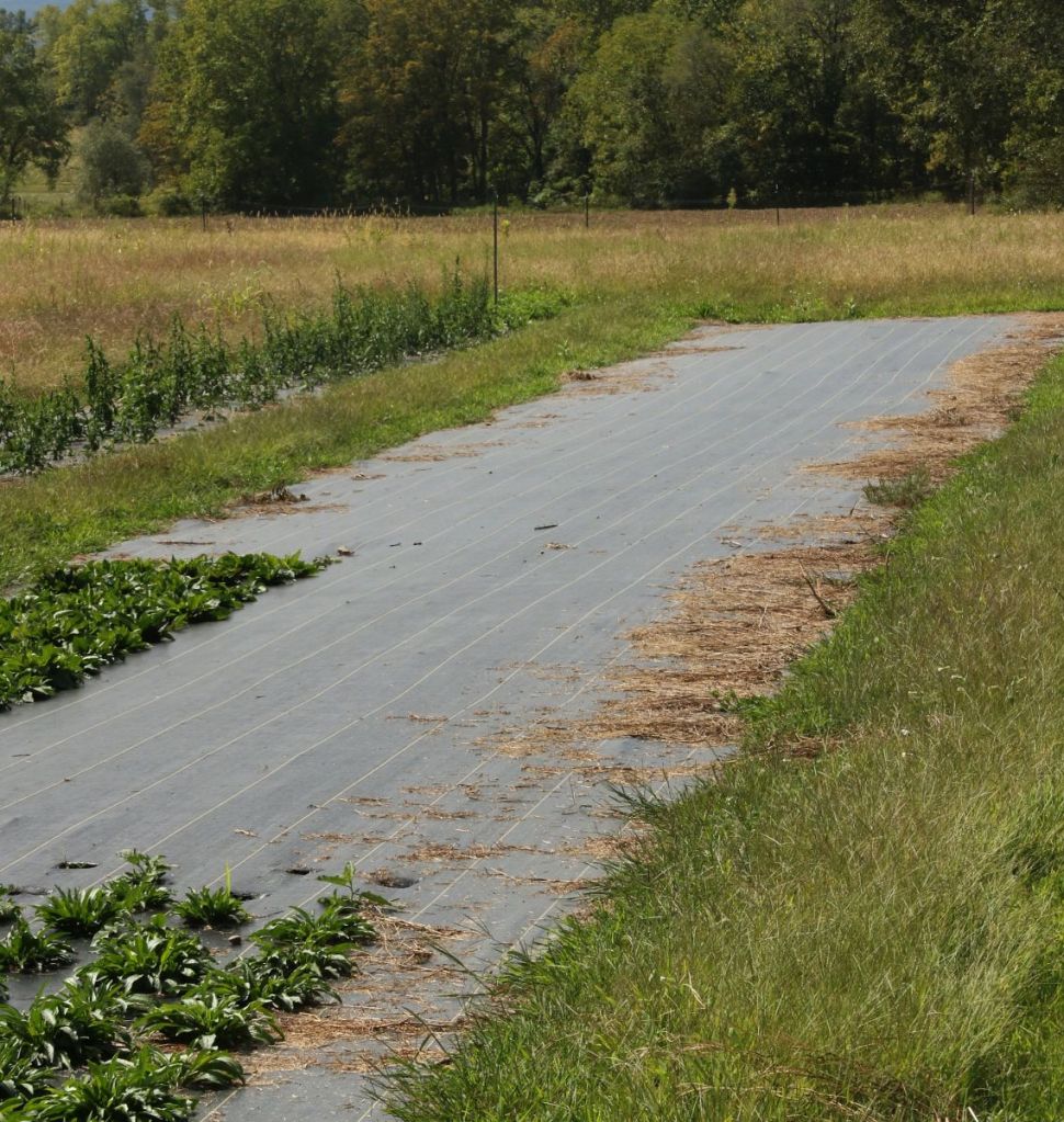
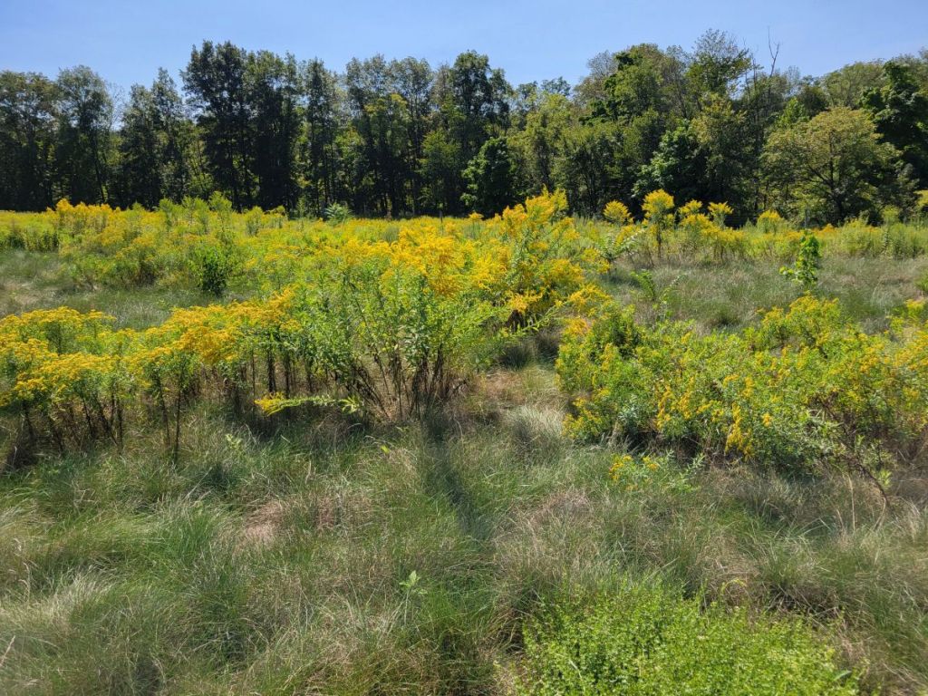
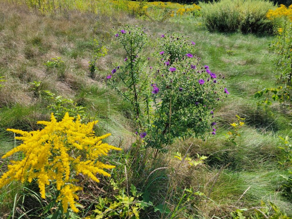
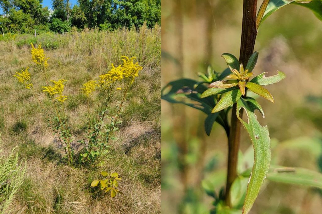
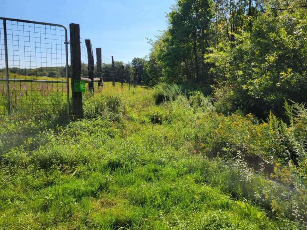
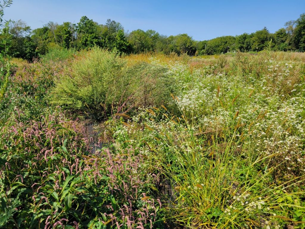
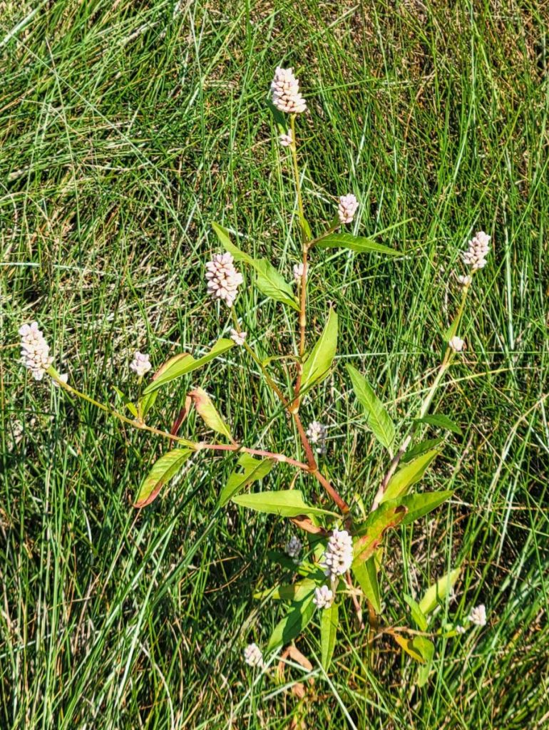
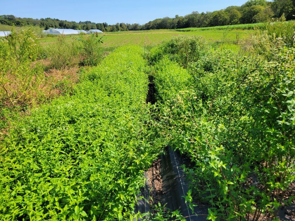
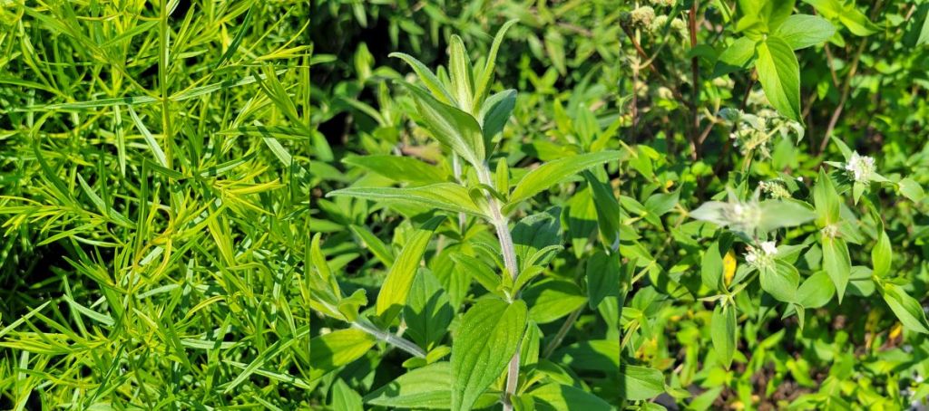
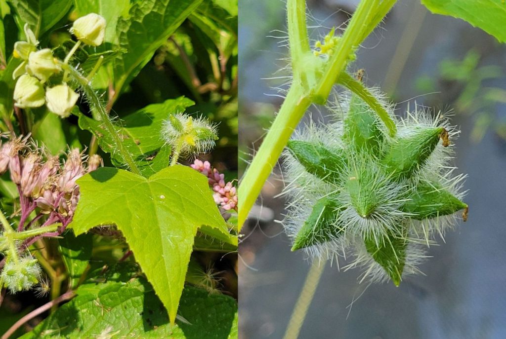
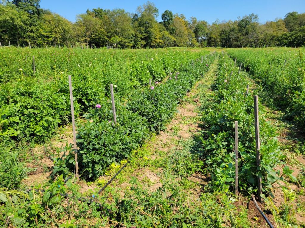
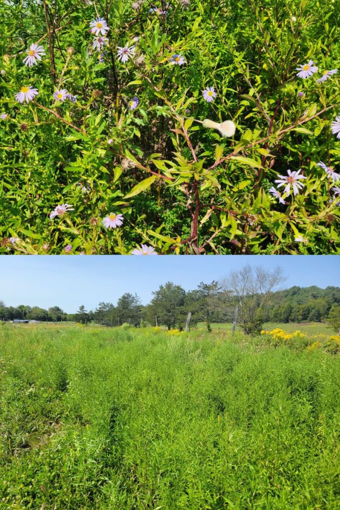
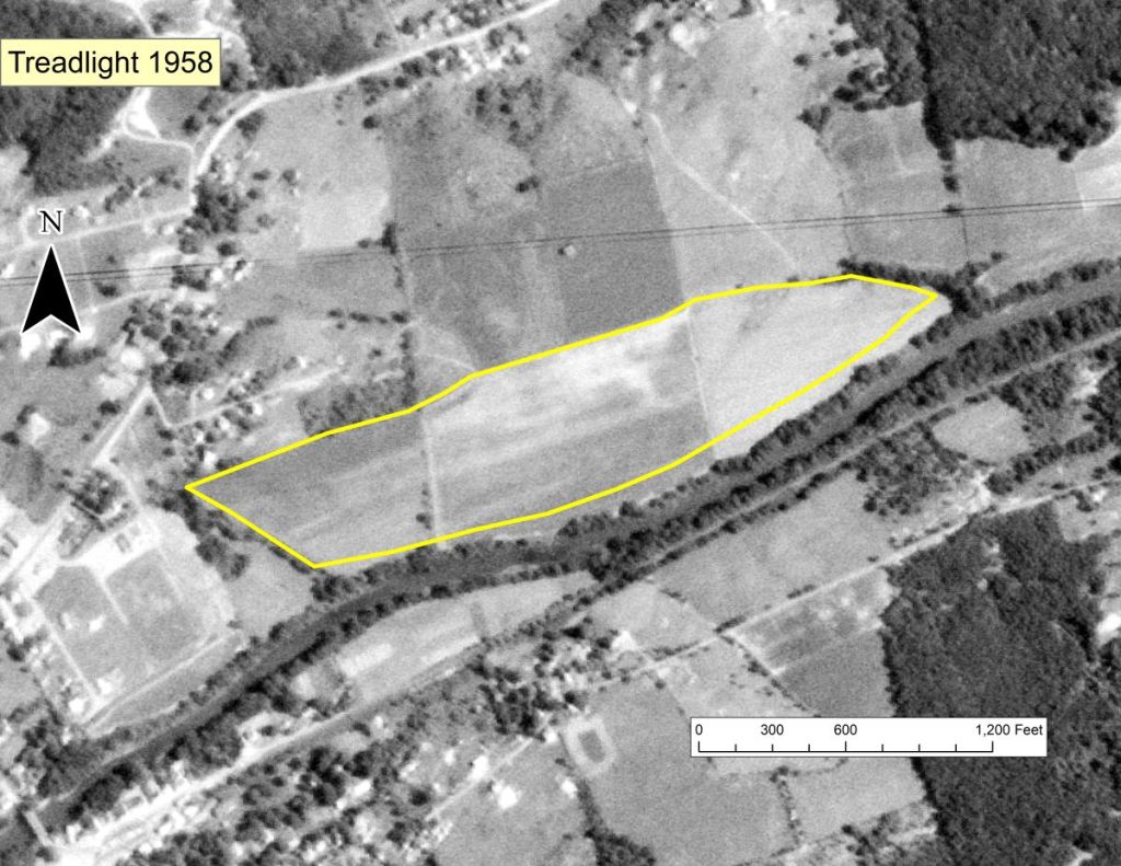
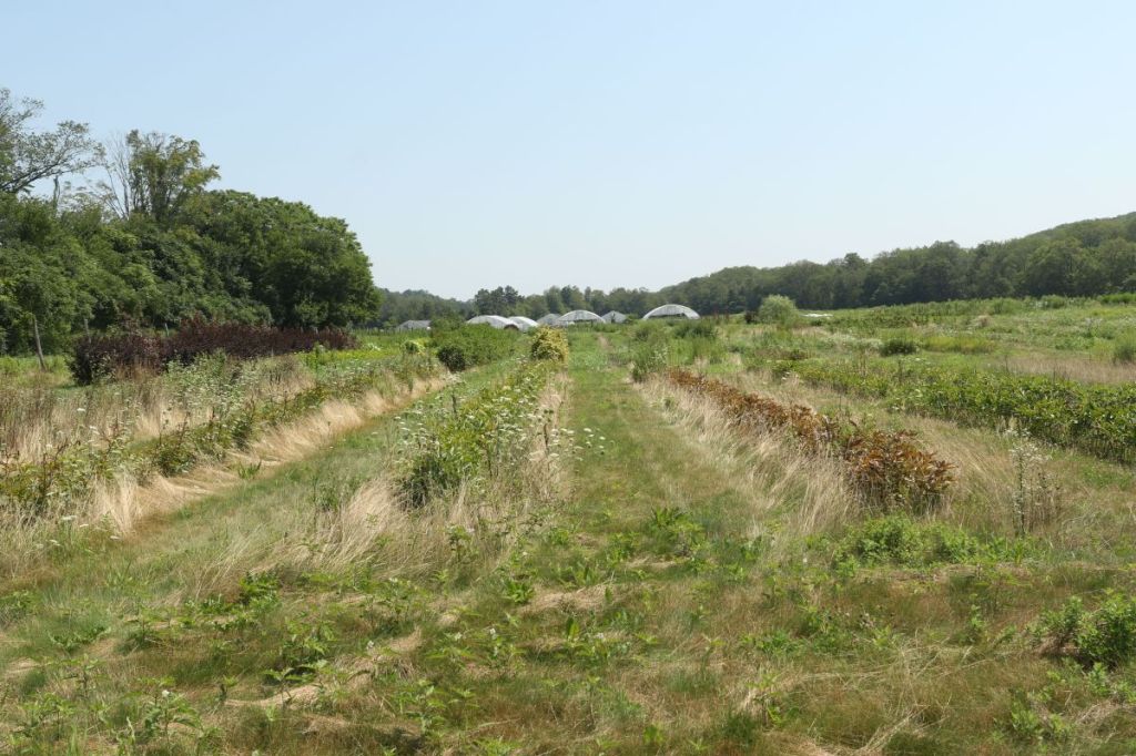
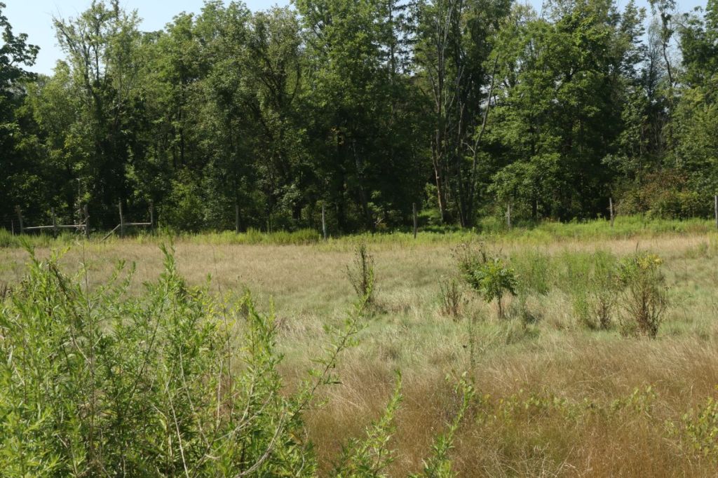
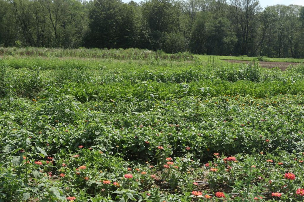
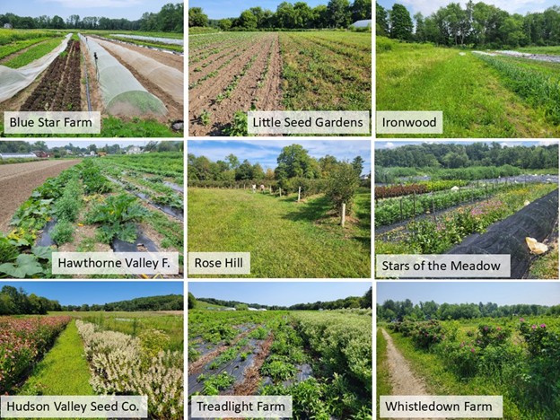
Flowers. After determining the study area at each farm, Claudia delineated survey units and classified them by general management regimes/habitat types. These included the categories: bare ground/plastic; cultivated flowers/woodies; cultivated, other; managed wildflowers; mature fallow; fenceline; mature cover crop; mature field edge; mowed; wild (Figure 1).

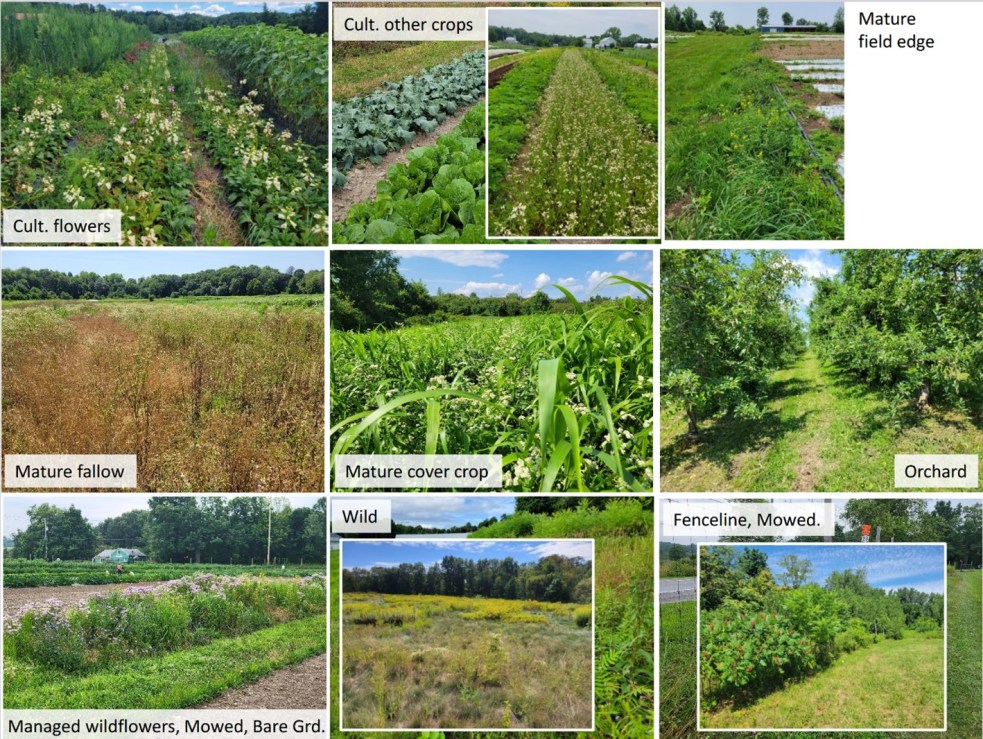
composite of various on-farm management regimes

Figure 1. Examples of the management regimes represented in our study

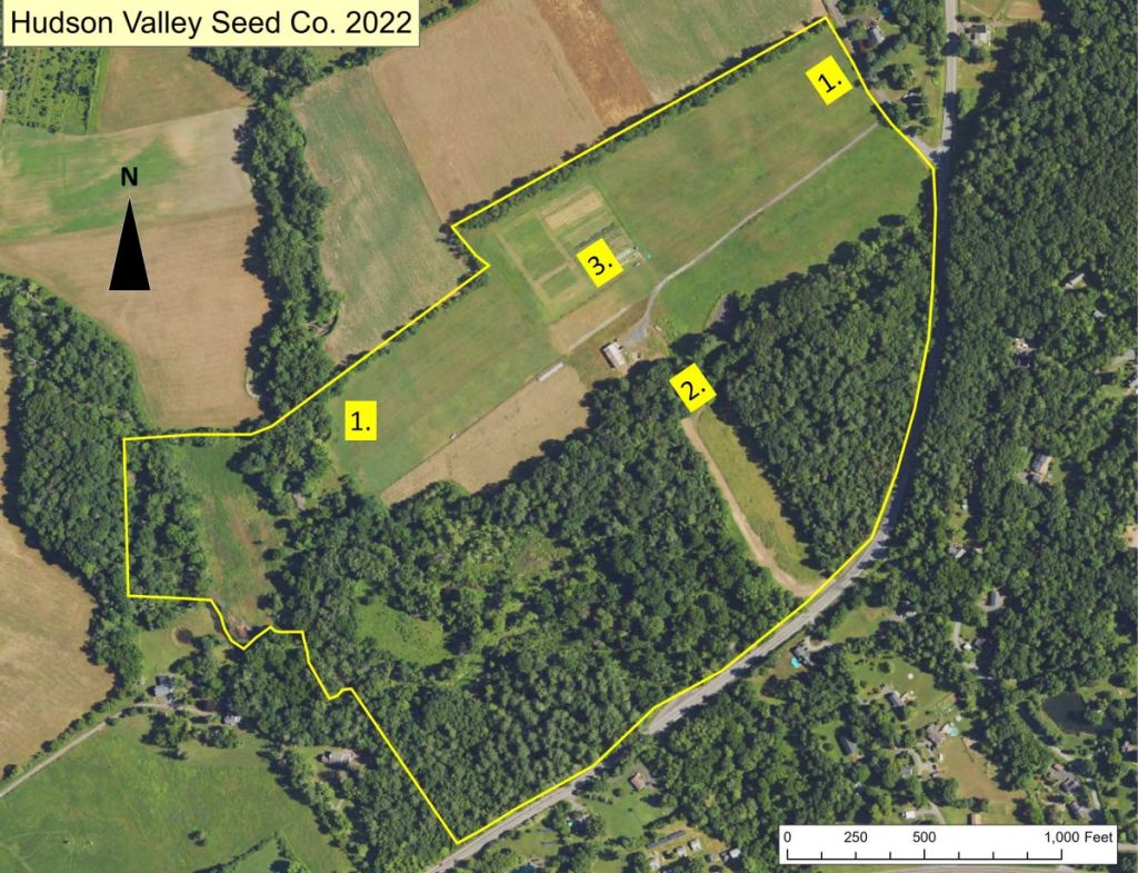
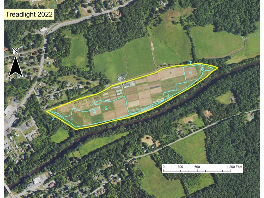
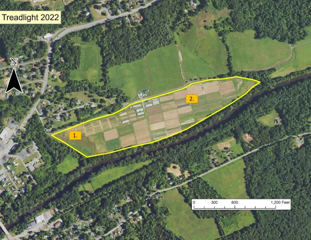
It is important to point out that we did not attempt to standardize the size of the study areas and number of survey units across farms. They were largely determined by practicality, the desire to include a variety of management regimes, the field conditions and our energy level during the first survey, and sometimes the preference/curiosity of the farmer. As a result, the study areas ranged from 1.6 acres to 10.4 acres in size and contained between 14 and 37 study units (Figure 2).

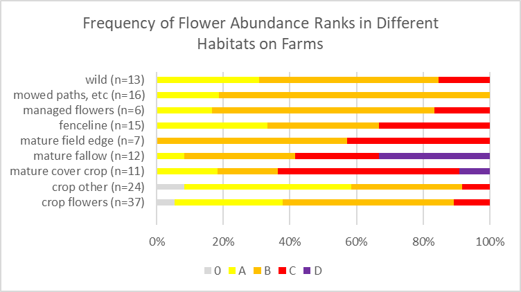
Within each survey unit, flower species present were noted, and they were given an abundance rating reflecting their abundance within the survey unit as a whole. We used four ranks, A-D to indicate increasing flower abundance. We also noted if there were no flowers in a unit. Each survey unit was also given an overall flower abundance rating considering all flowering species present. Back in the office, the various survey units were delineated on aerial images and the floral data were associated with the corresponding spatial data. This allowed the mapping of the abundance of individual flower species, overall flower diversity, overall flower abundances, and the diversity of such flower classes as wild-growing and cultivated.

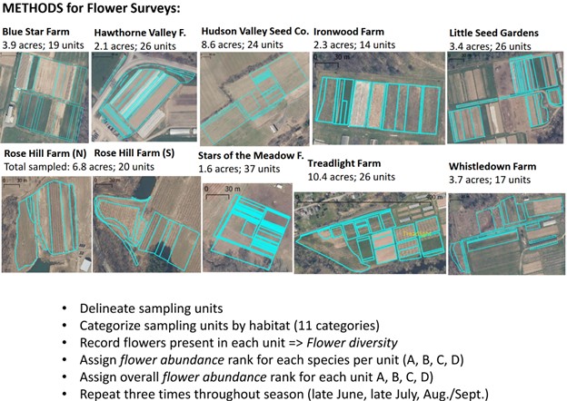
summary of plant survey methods and their characteristics at each farm

Figure 2. A visual comparison of the study areas and survey units of the nine farms and a summary of the methodology for the flower surveys

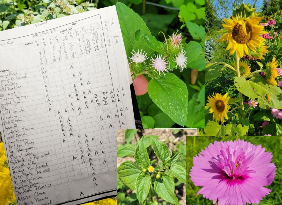
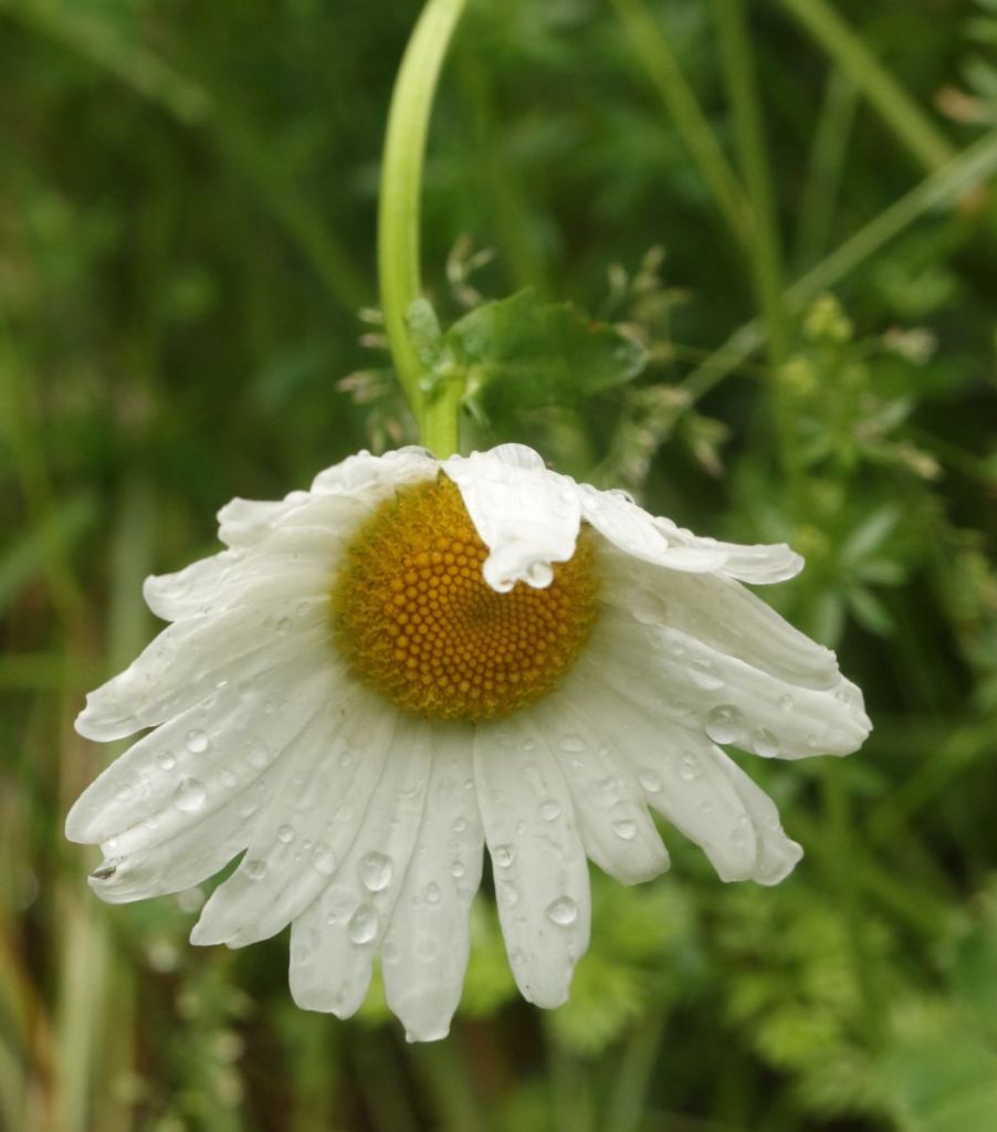
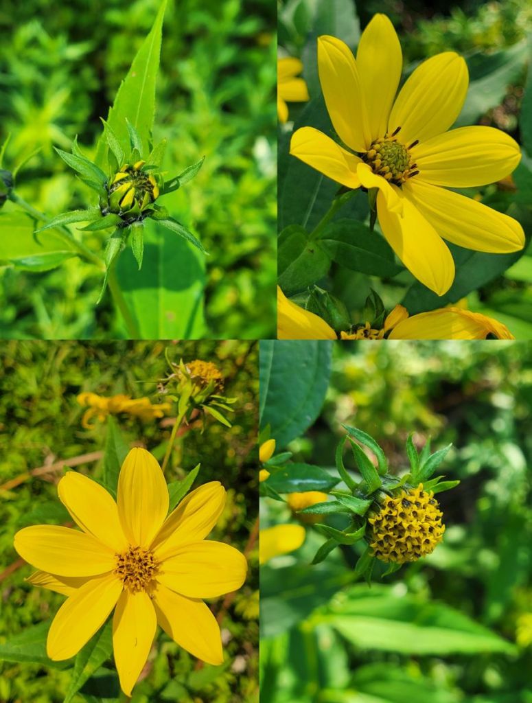
Figure 3. Example of a field data sheet used in the flower surveys and some of the flowers encountered during these surveys (clock-wise from top left): Clustered Mountain-mint, a budock species, Common Sunflower, Garden Cosmos, a quickweed species, and a goldenrod species.

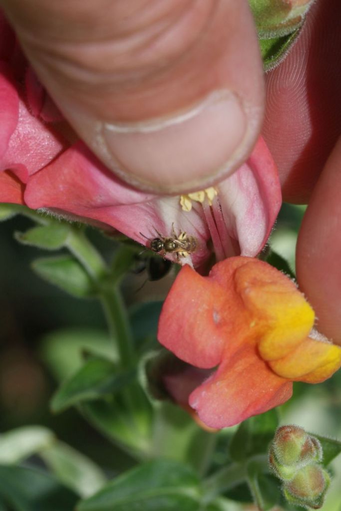
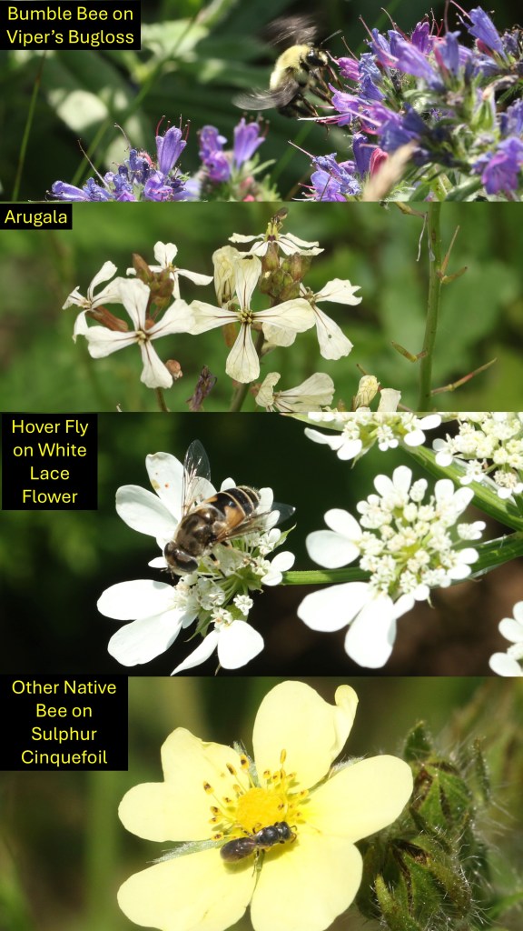
Flower Visitors. Conrad took his cue from the flowers that Claudia identified and tried to visit, if not all flower species, then at least the most common ones. For each flower species observed, an attempt was made to spend five minutes inspecting new flowers of the focal species. If the flowers were organized in a bed, then this meant walking down the bed, with eyes moving from flower to flower as the presence or absence of a flower visitor was determined. A stopwatch was used and only time spent inspecting new flowers was included in the timed observations; if Conrad was distracted or if a given flower was discontinuously distributed, timing stopped during the non-observational activity (e.g., taking photos) or during the walk to another flower of that species. Sometimes low flower availability meant that it was not practical to fill five minutes with flower observation; in such cases, the total period of actual observation was recorded. As alluded to earlier, a few relatively crude taxonomic categories were used to tally flower visitors in most cases. For bees, the tally categories were Honey Bee, Eastern Carpenter Bee, bumble bee and “other bee”. However, Eastern Carpenter Bees were relatively few, and so are excluded from some analyses. Effort was made to ID unusual bumble bees and “other bees” was in part the sum of several other, more specific bee tallies including those of Hylaeus (the tiny masked bees), Green Sweat Bees, and Ceratina (the smaller carpenter bee). These added data are summarized in some ancillary analysis, but only the four aforementioned categories of bees were used for the core analysis. Other, non-bee groups included butterflies, wasps, and hover flies. Butterflies were usually identified to species, and some additional ID attempts were made of other flower visitors but, again, these are not included in the core analysis.

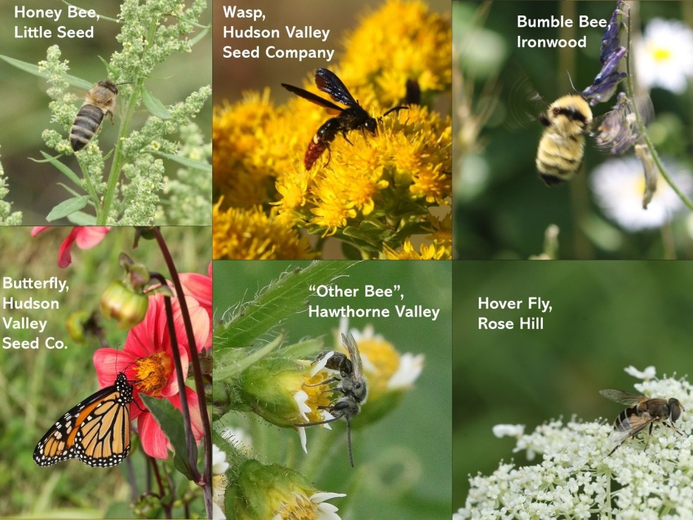
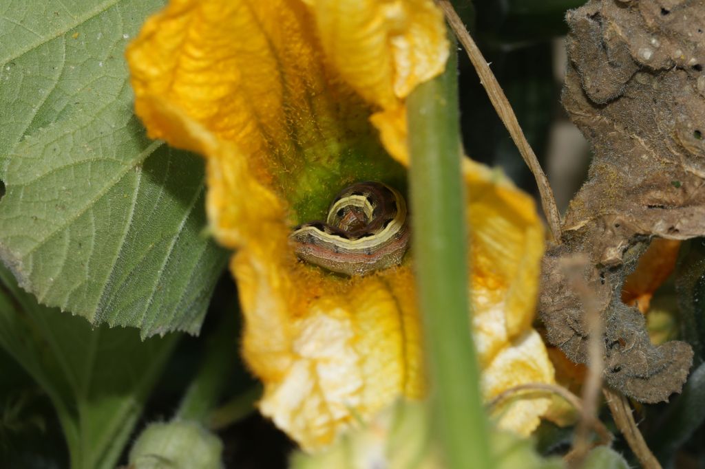
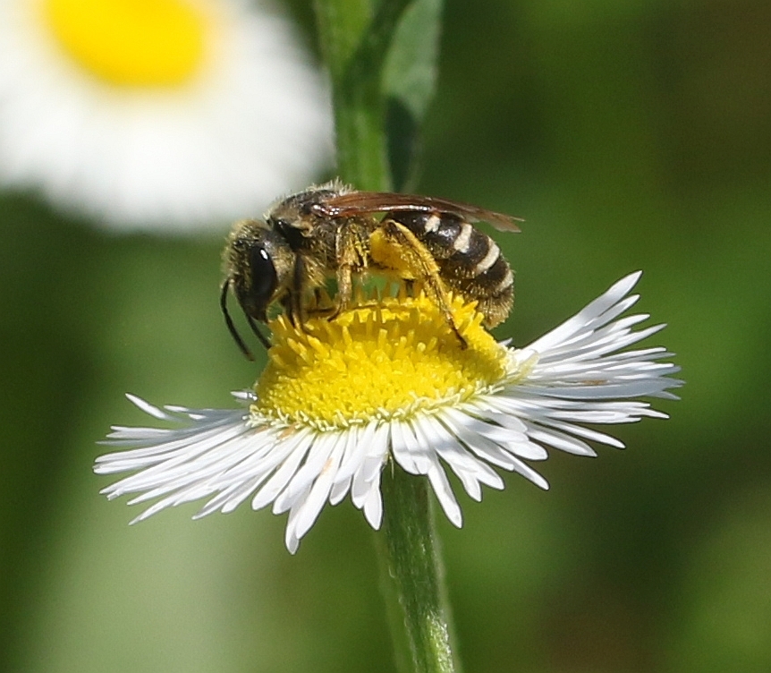
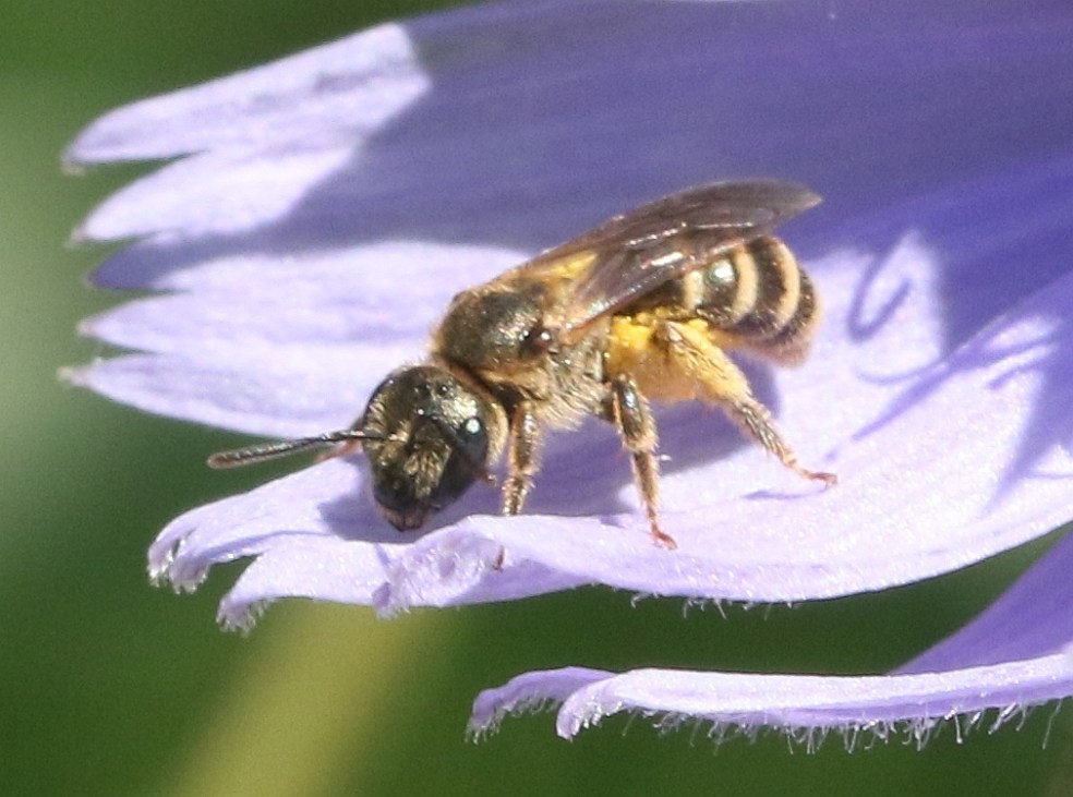
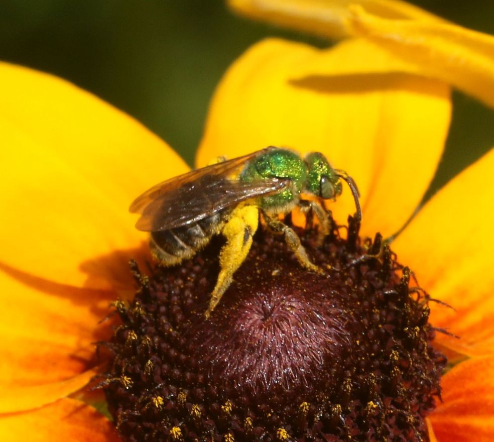
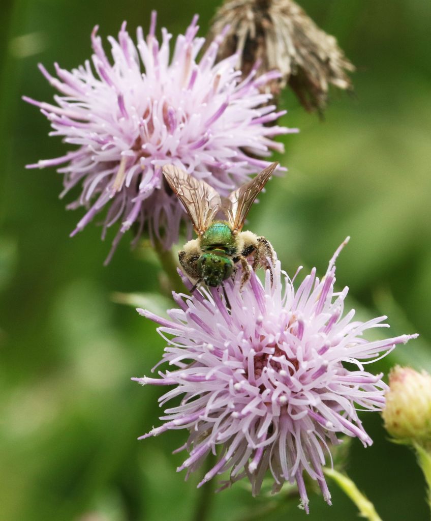
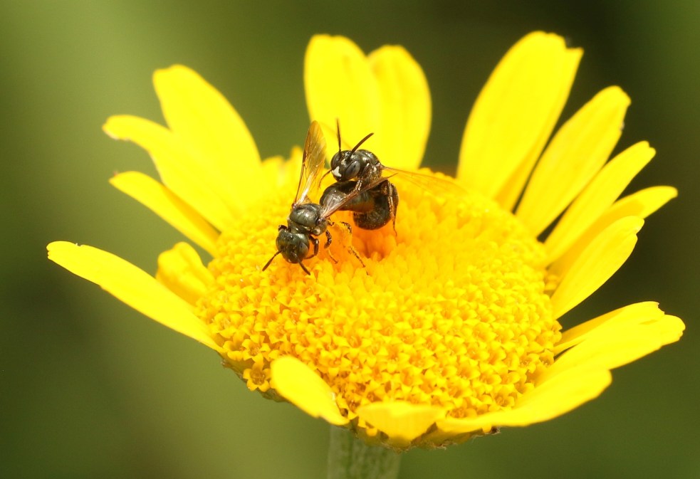
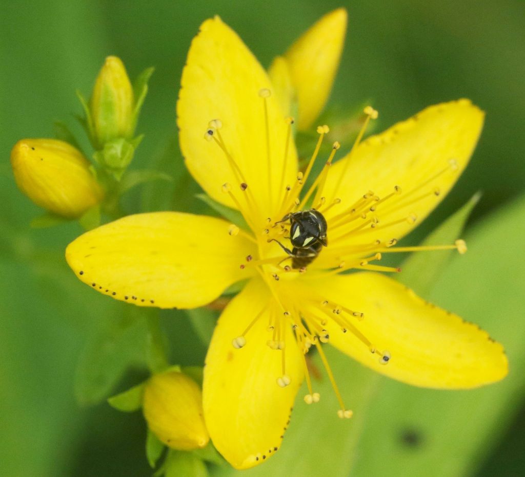
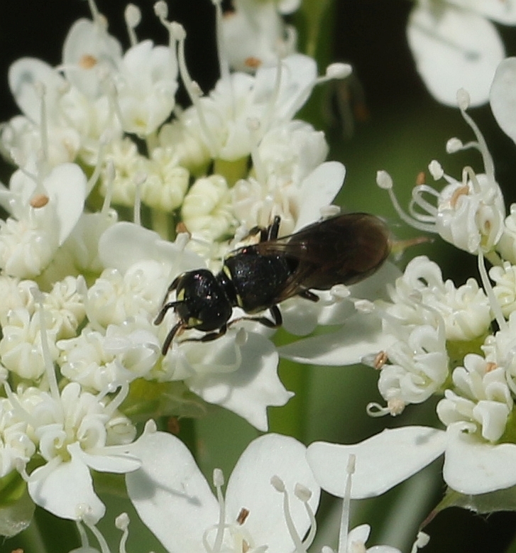
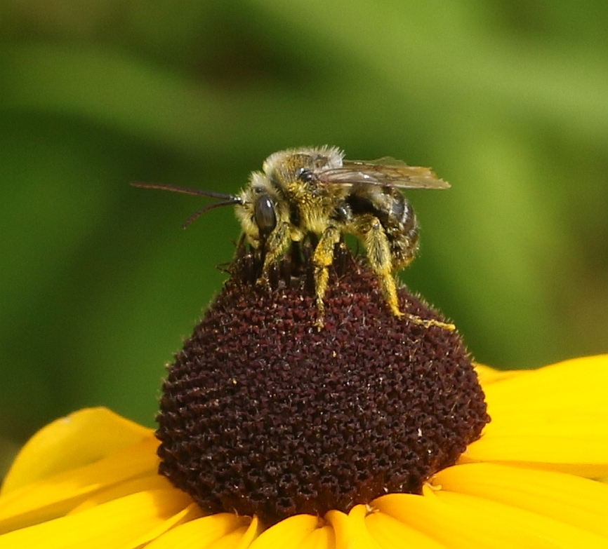
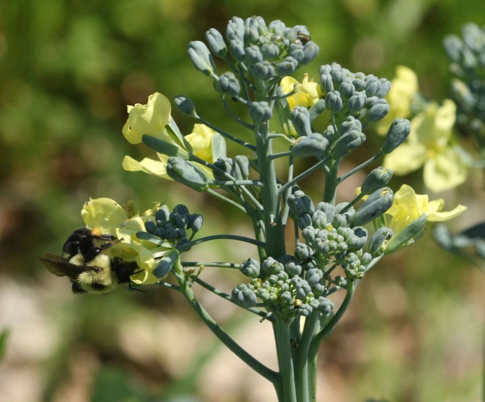
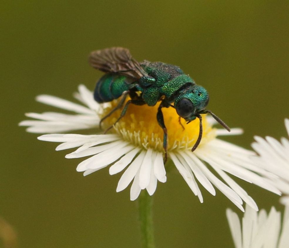
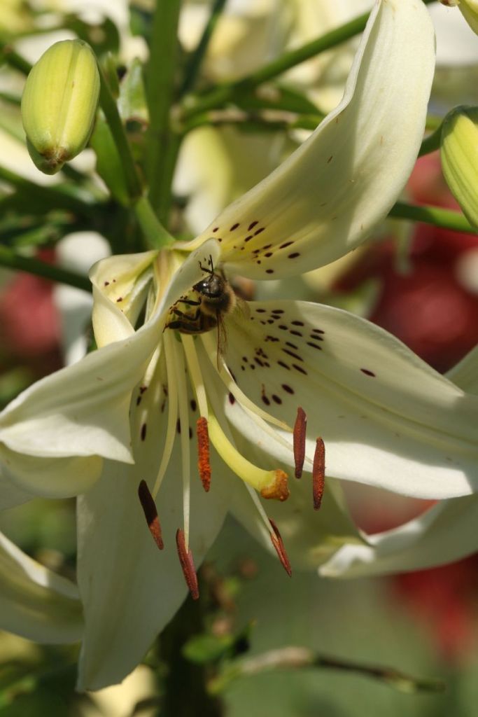
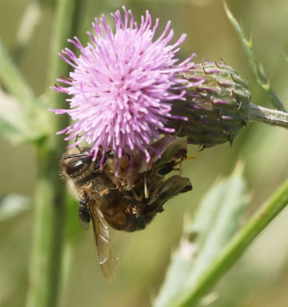
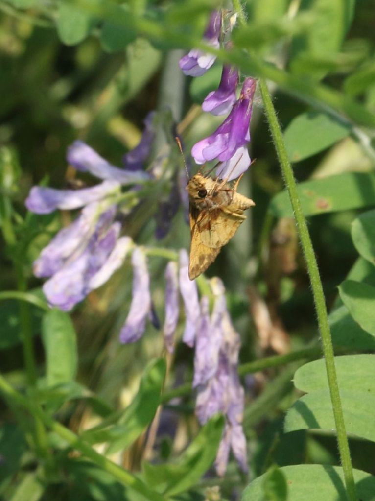
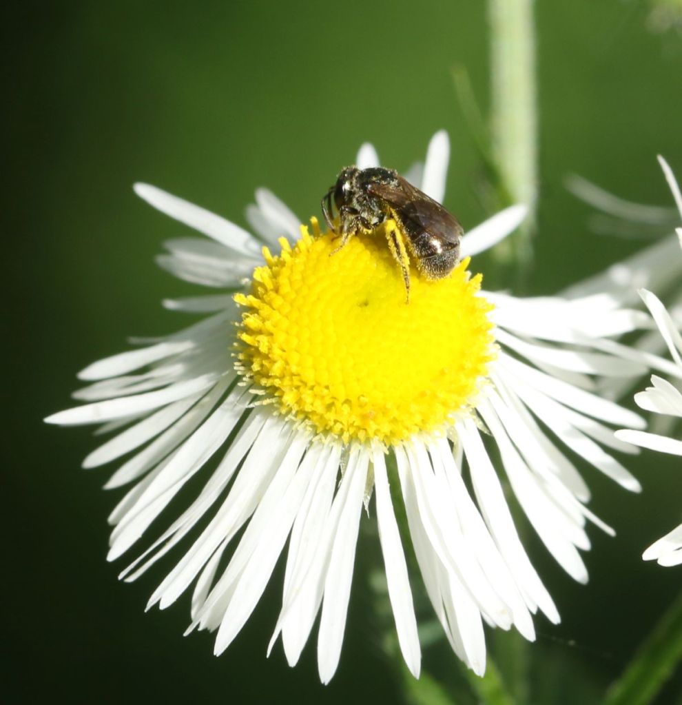
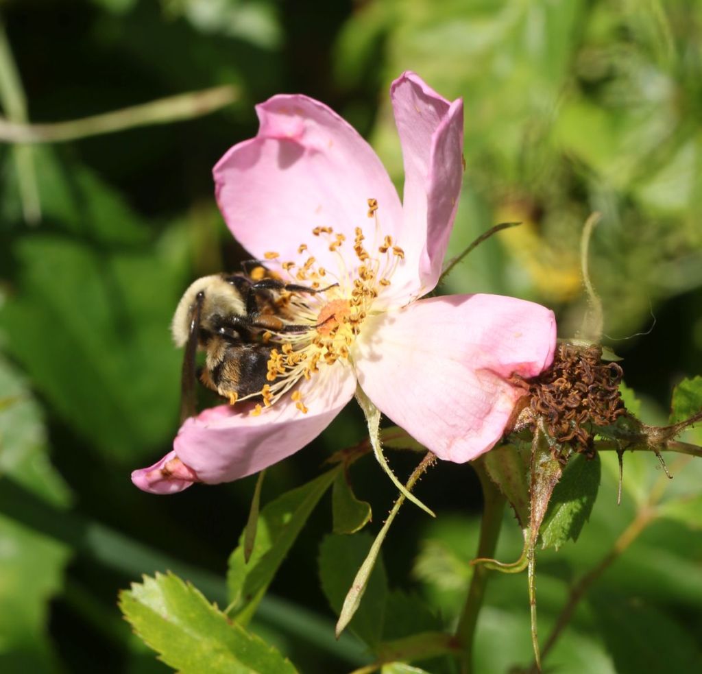
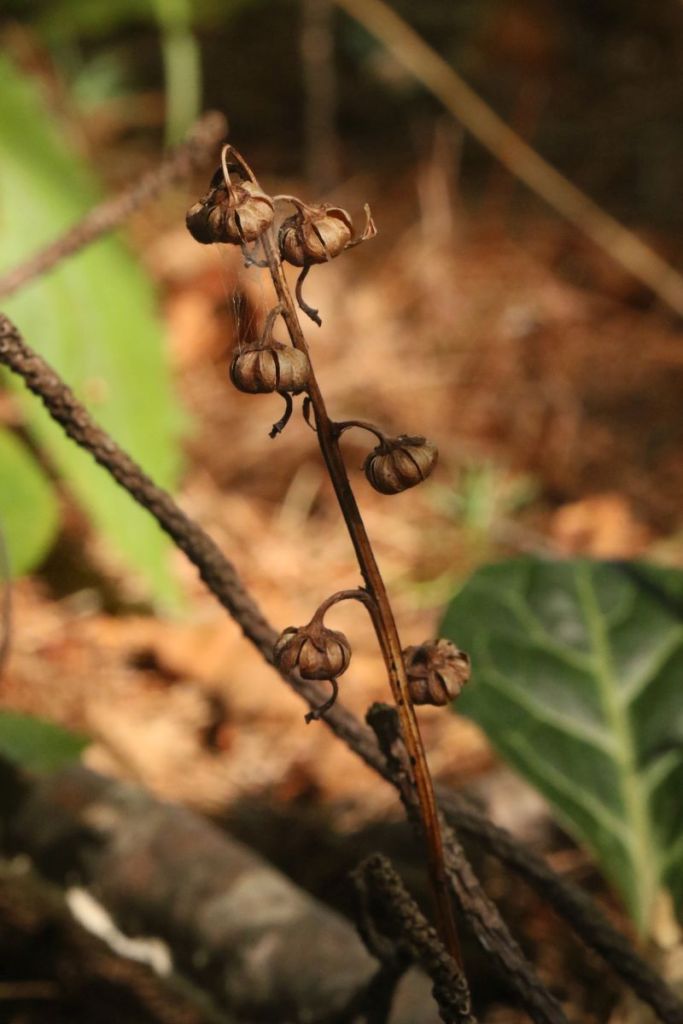
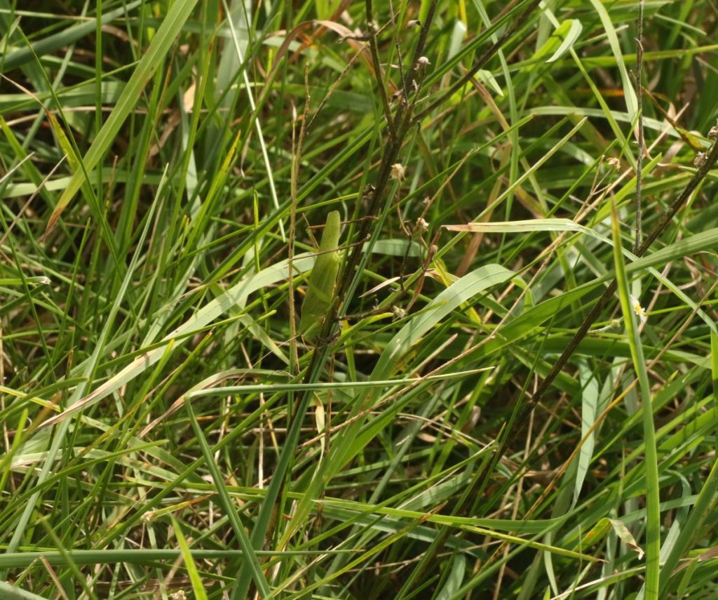
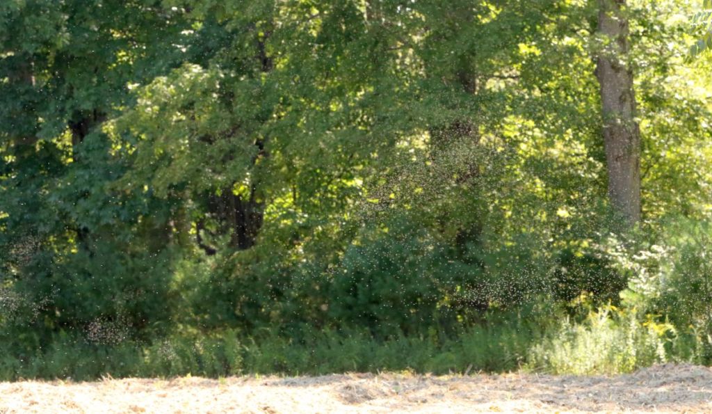
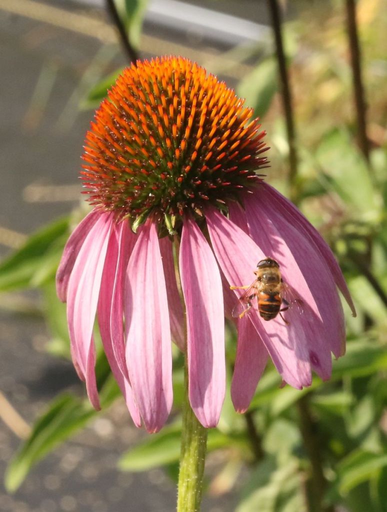
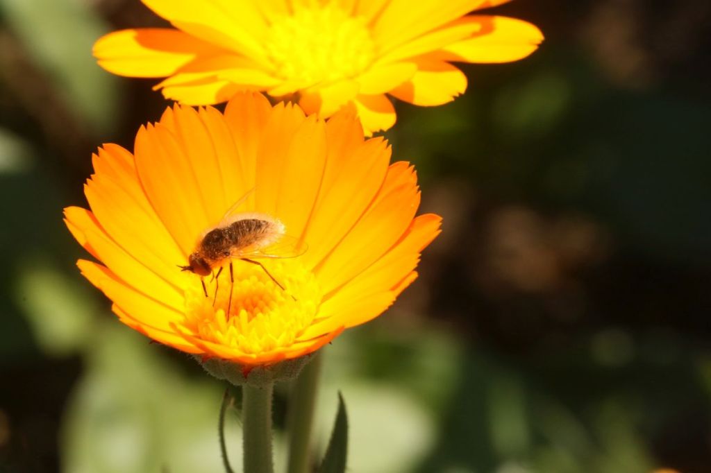
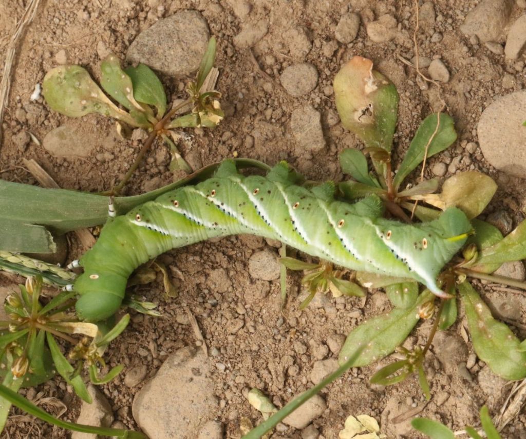
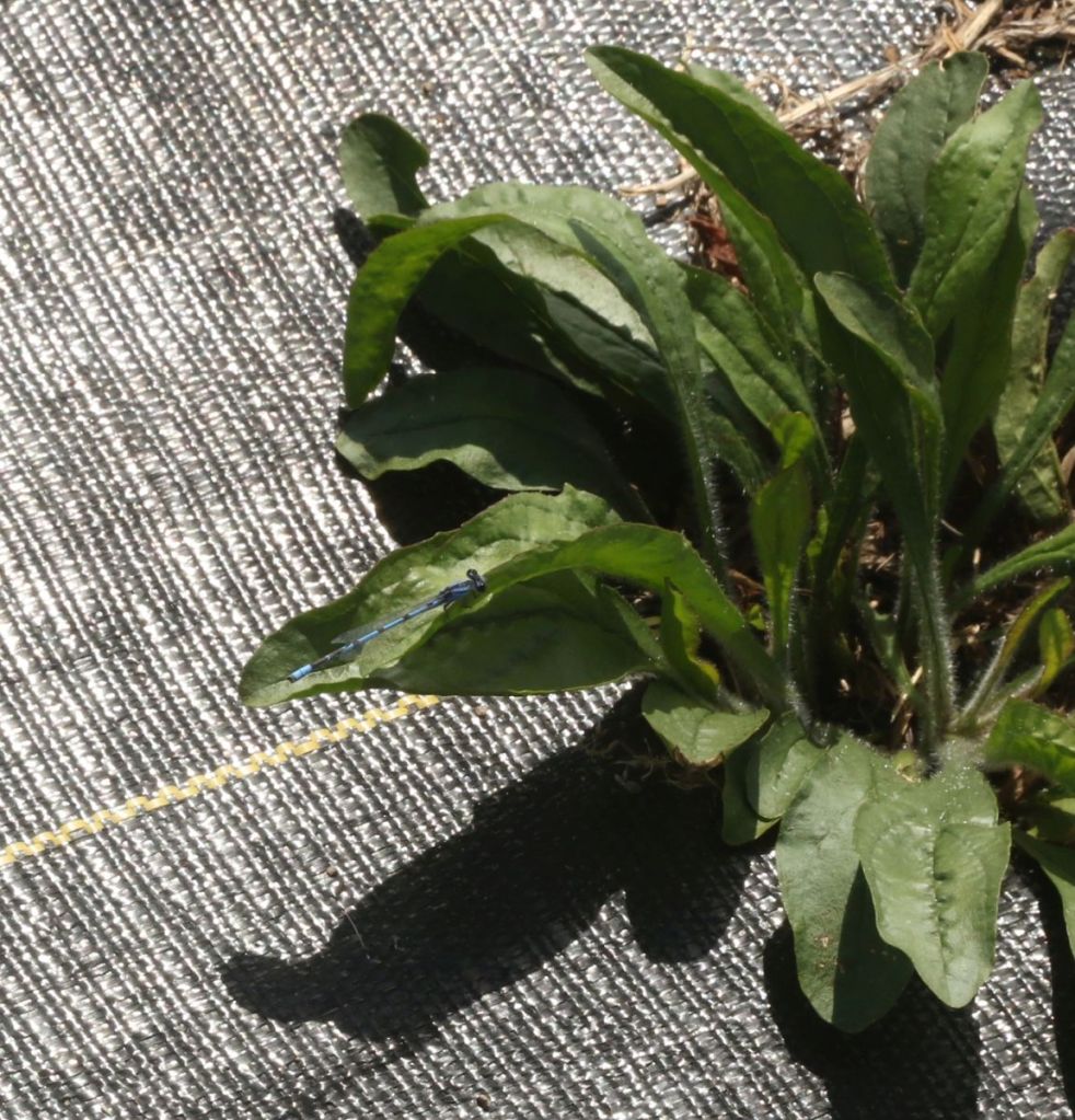
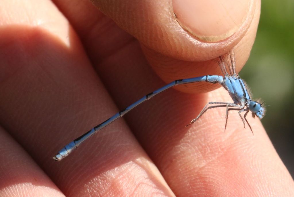
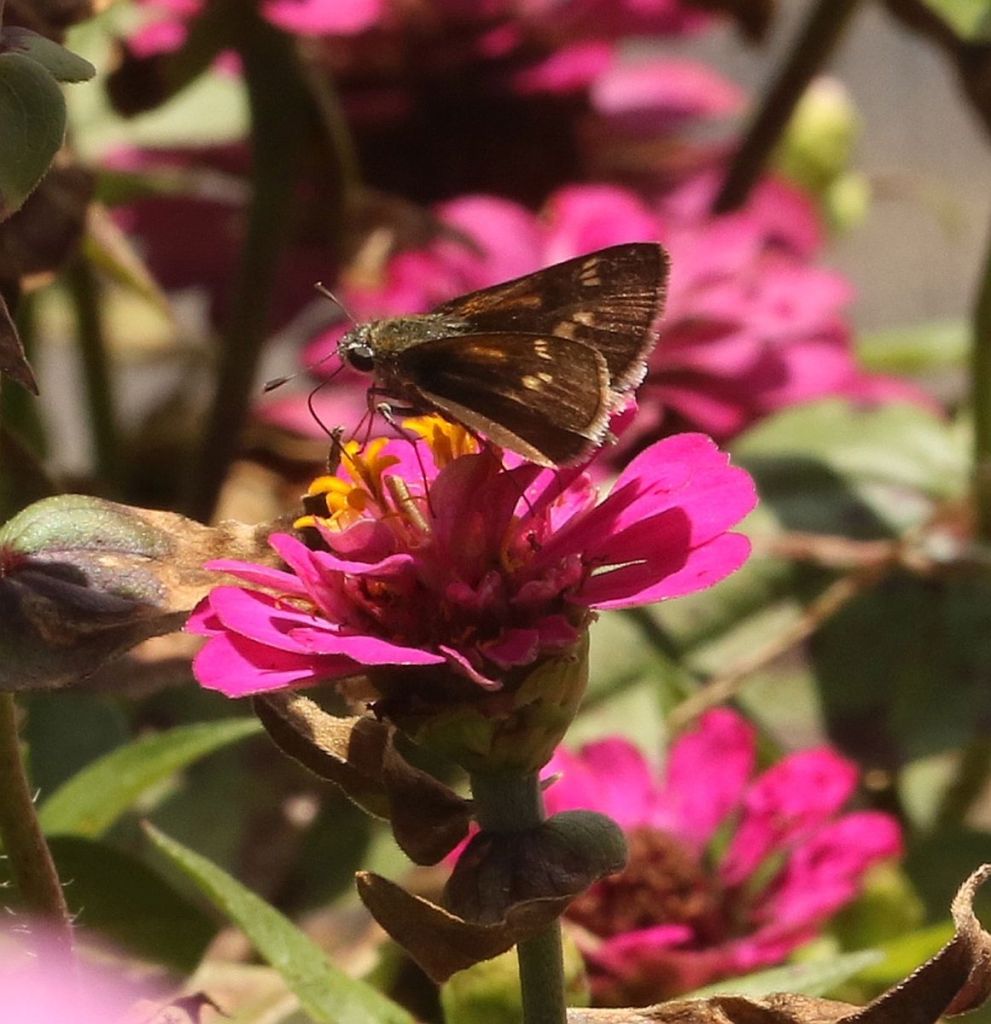
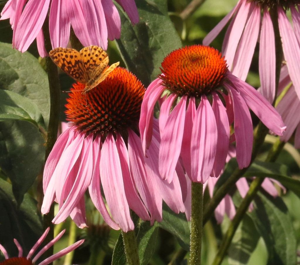
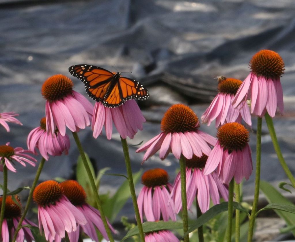
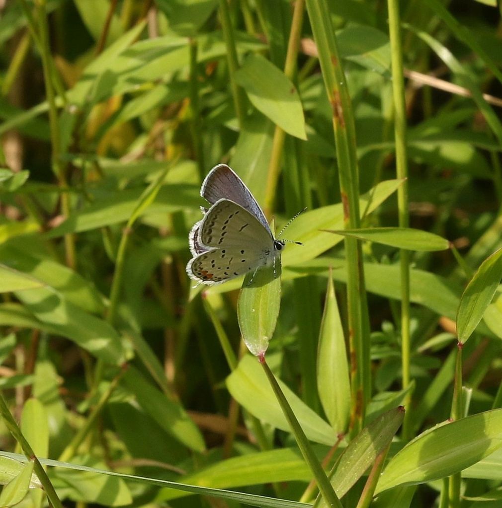
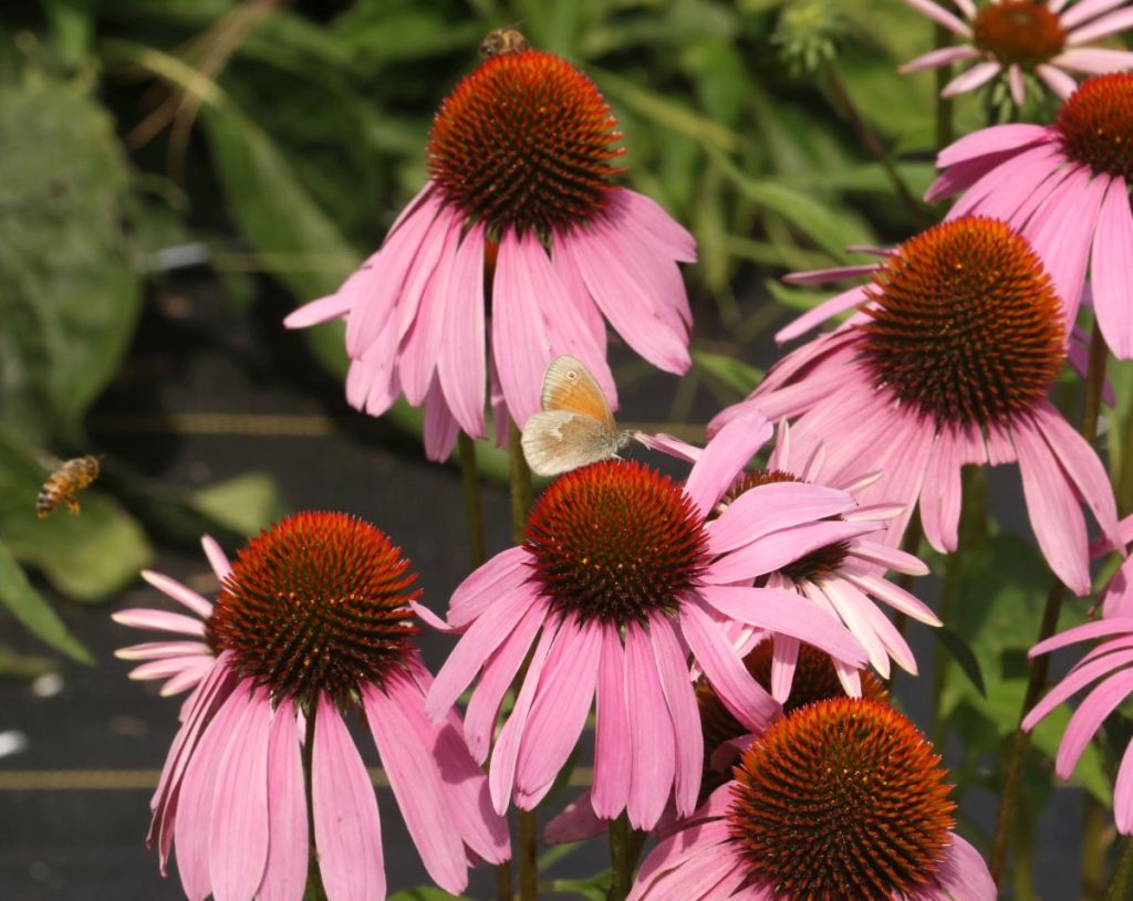
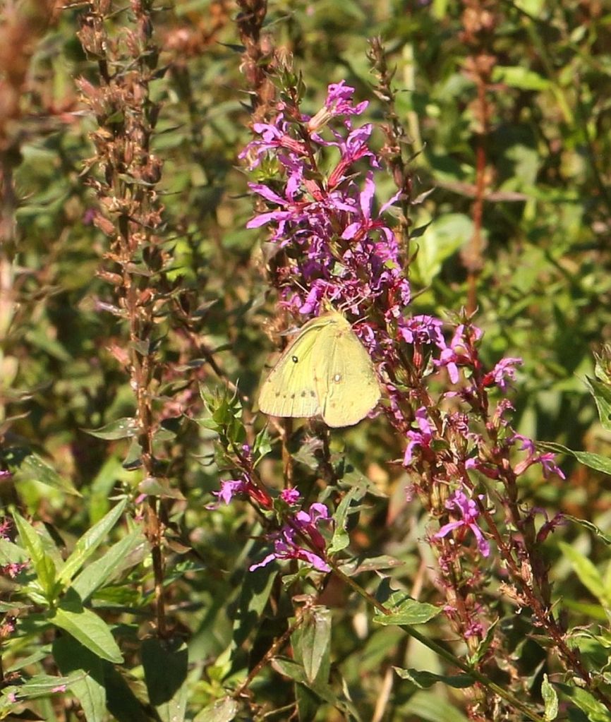
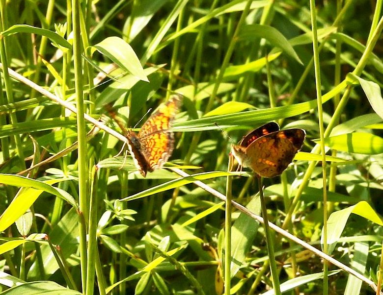
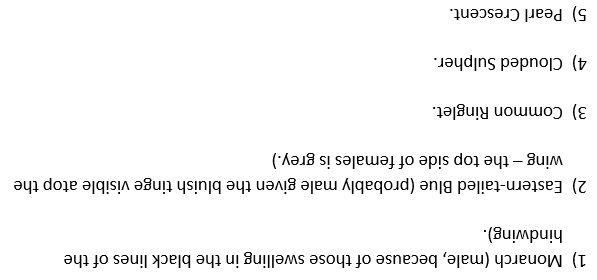
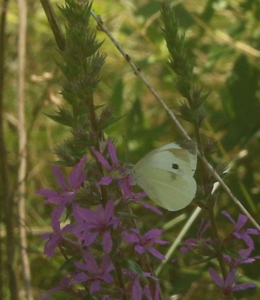
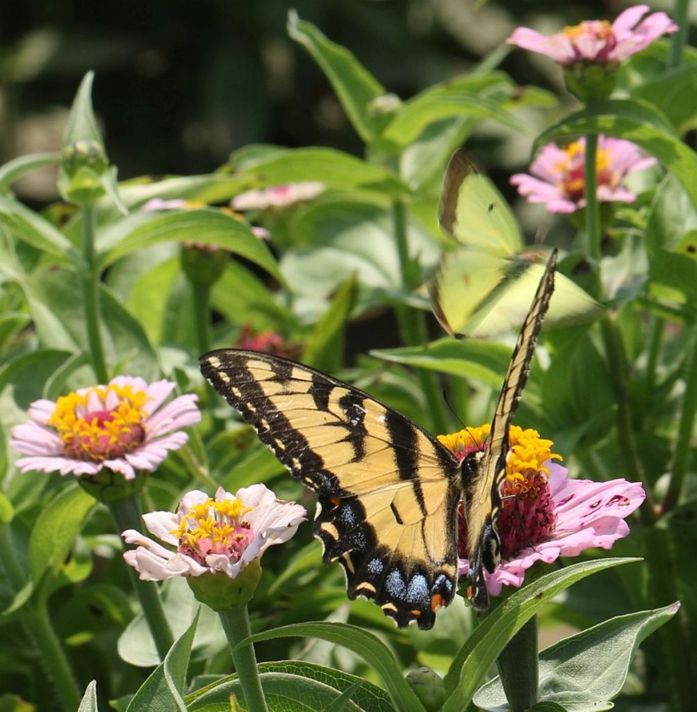
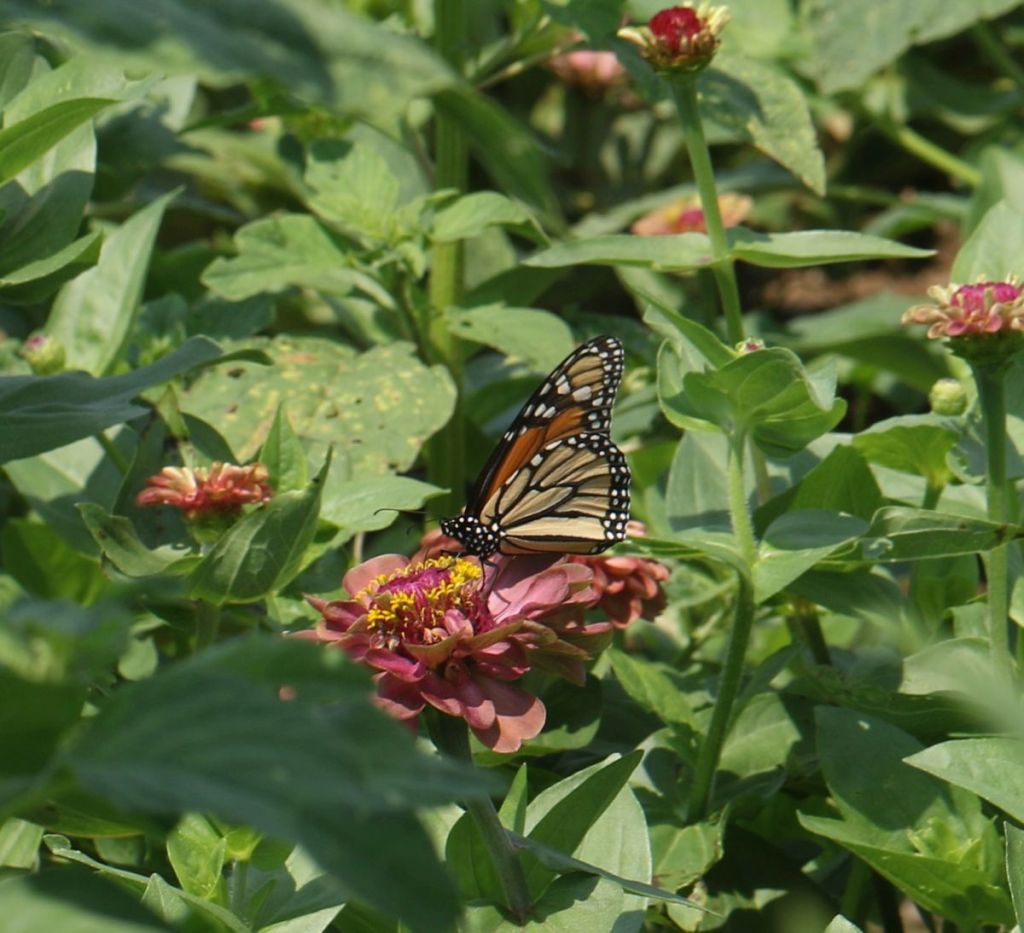
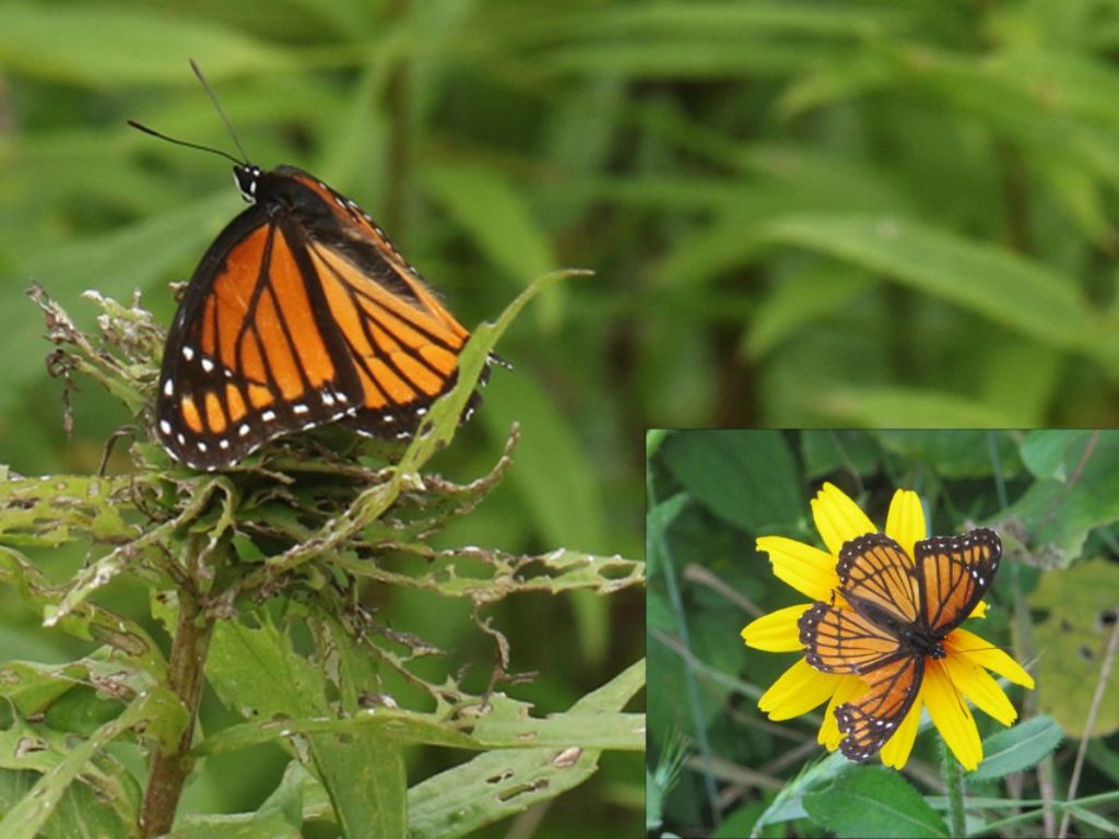
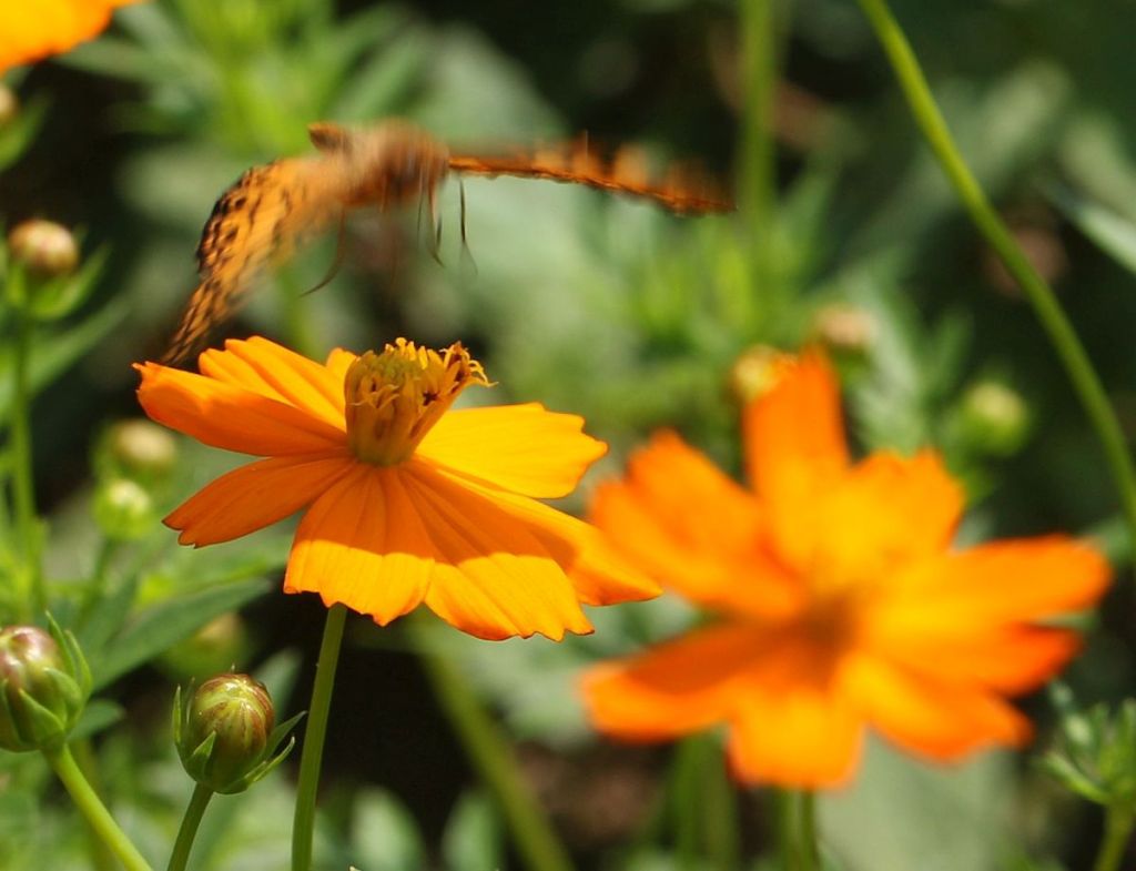
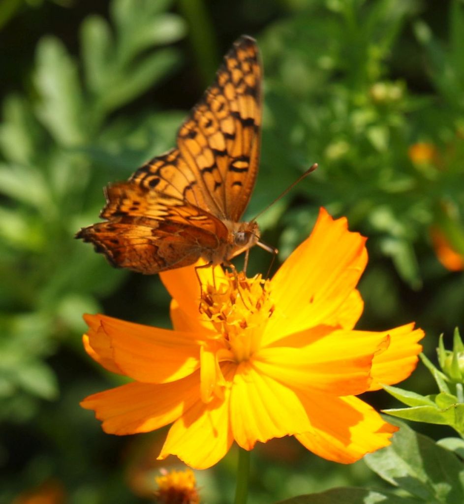
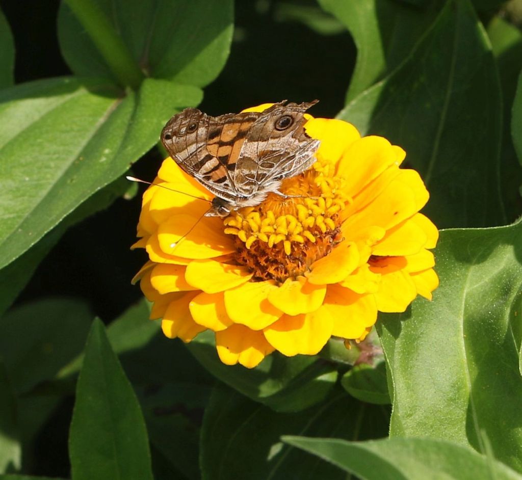
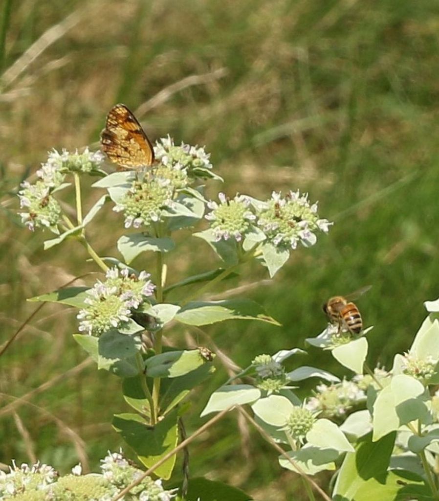
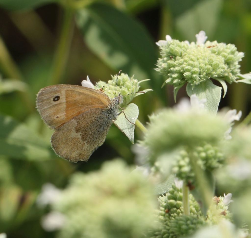
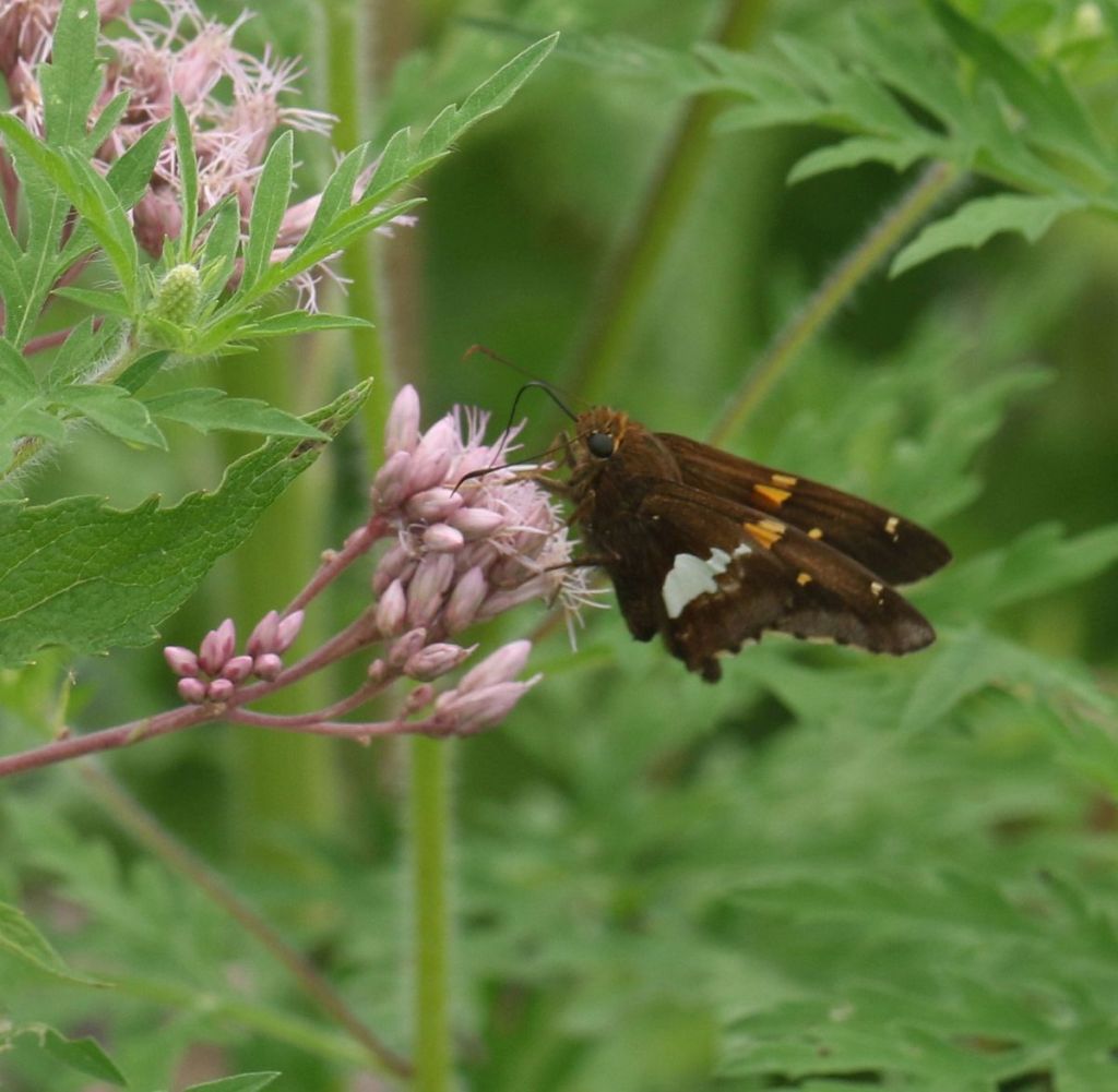
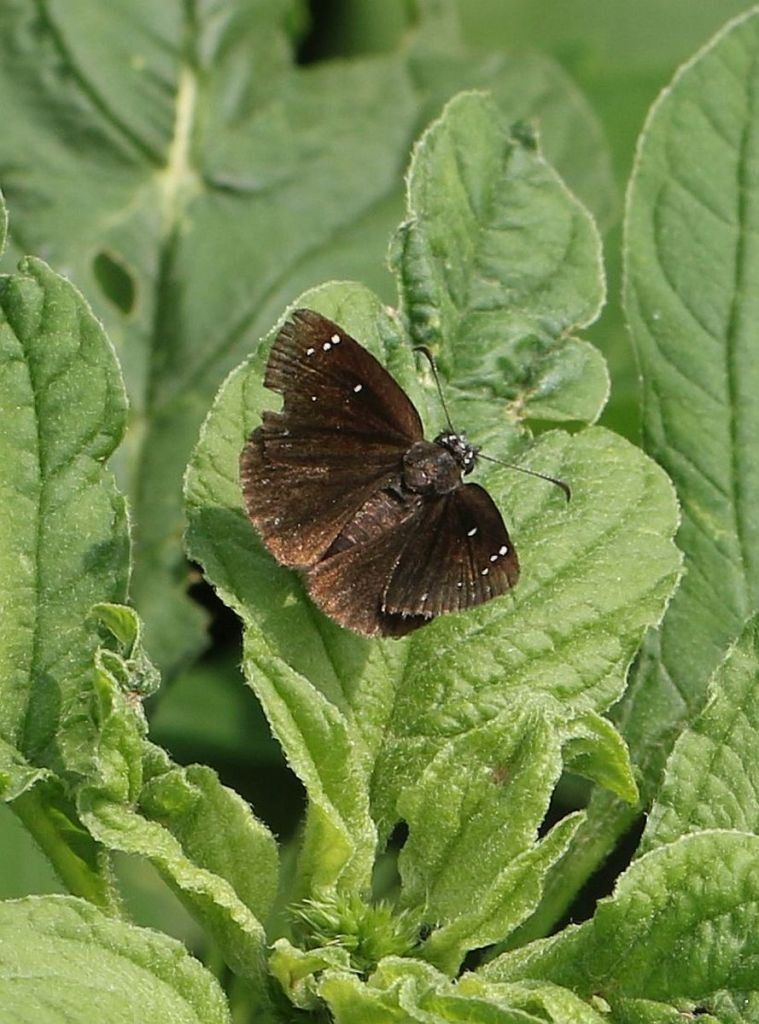
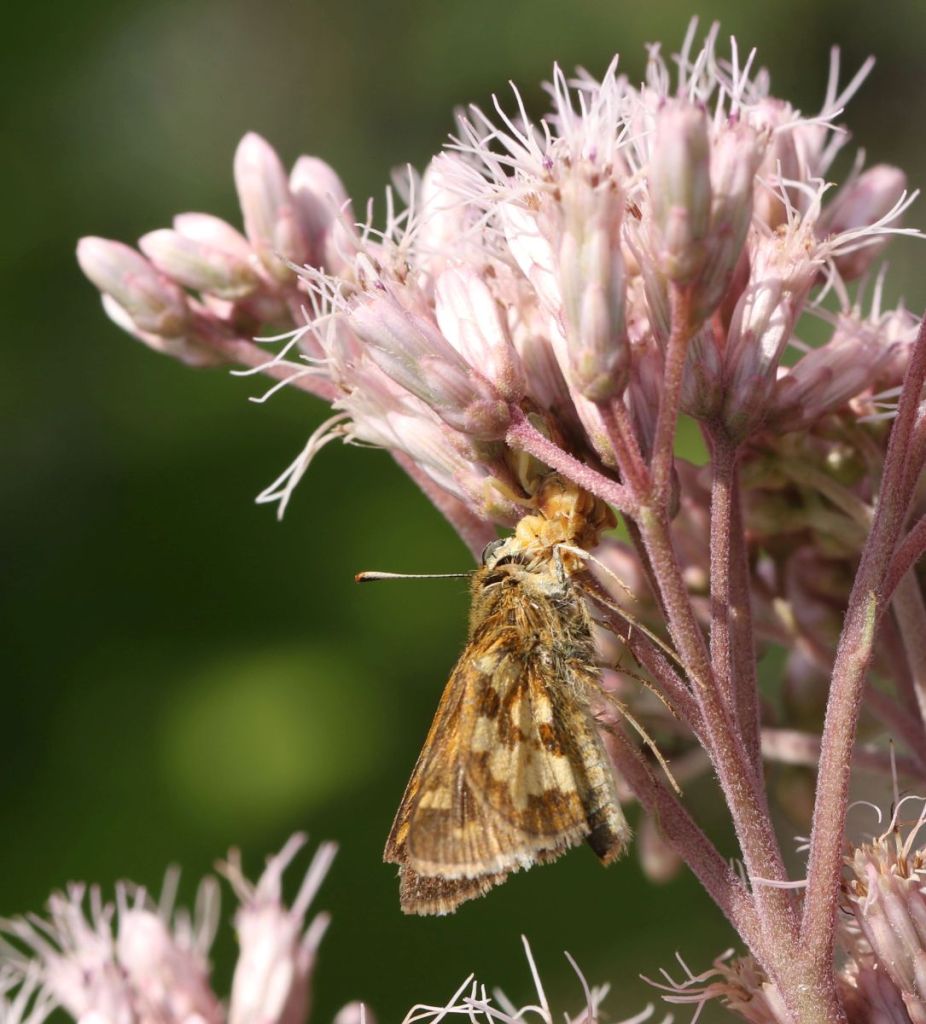
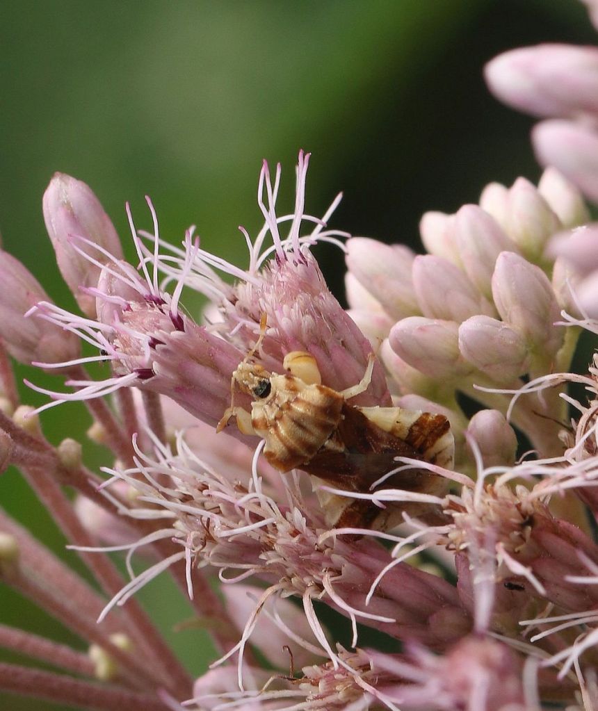
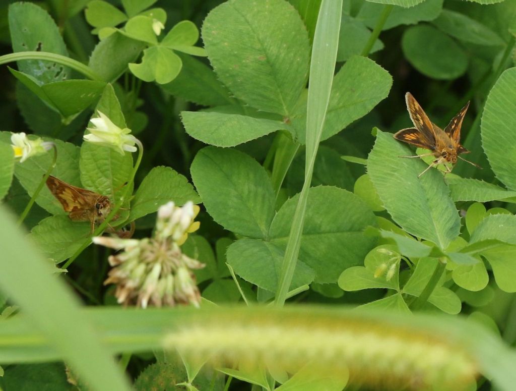
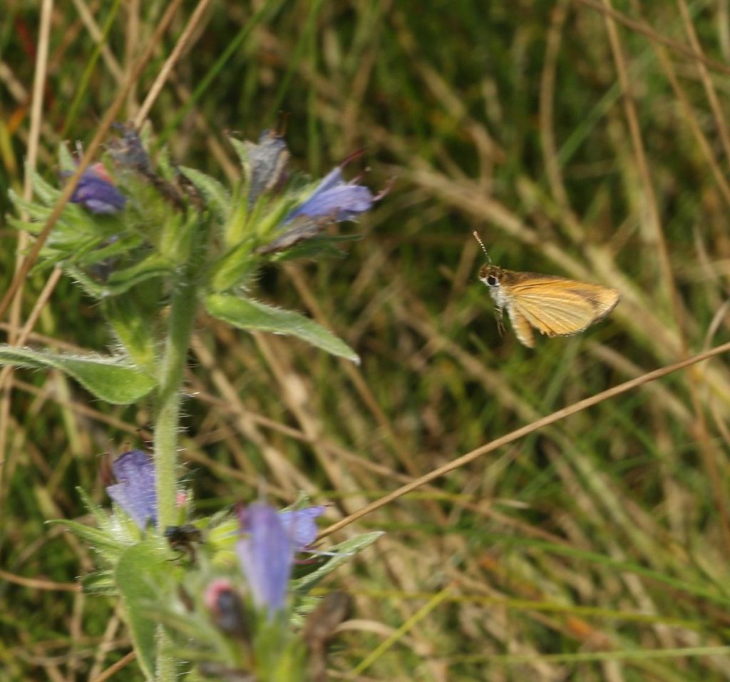
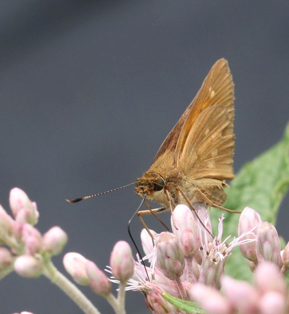
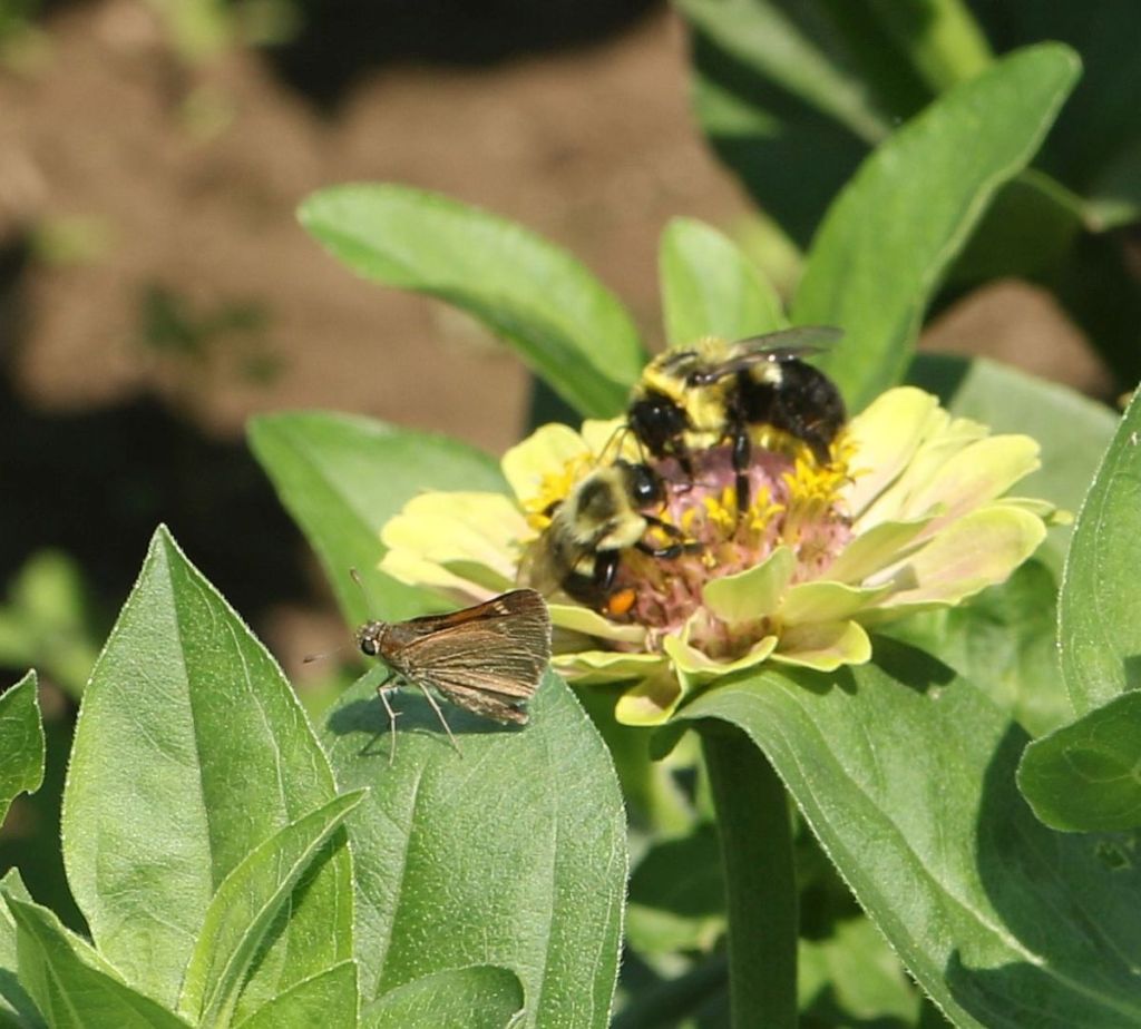
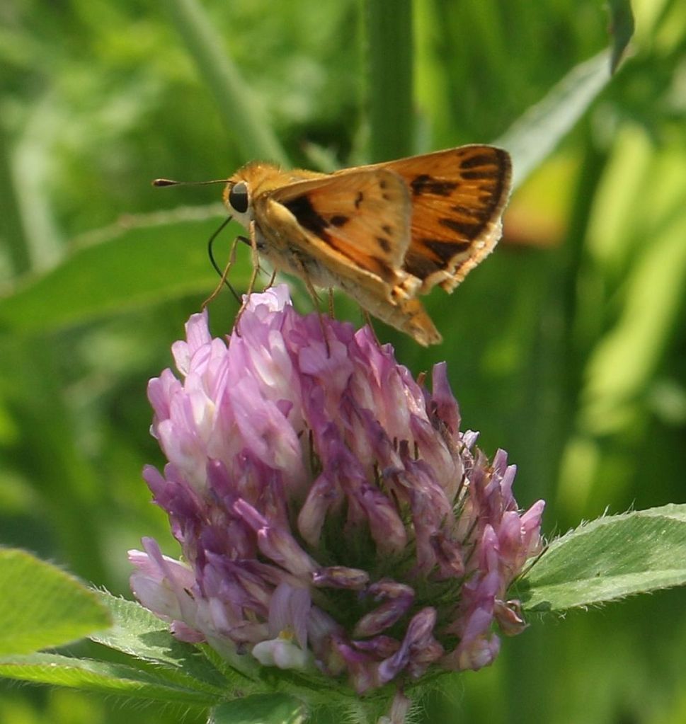
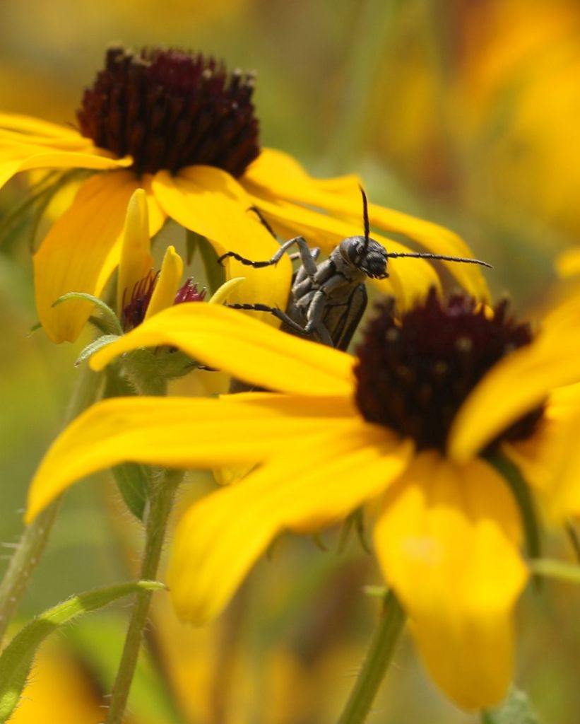
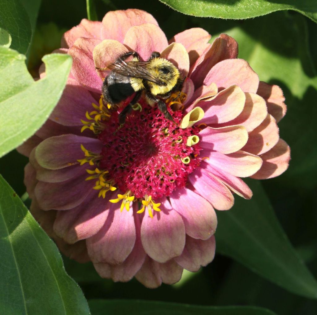
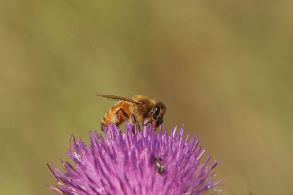
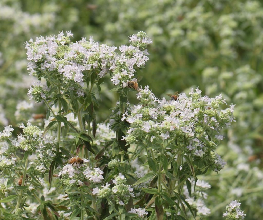
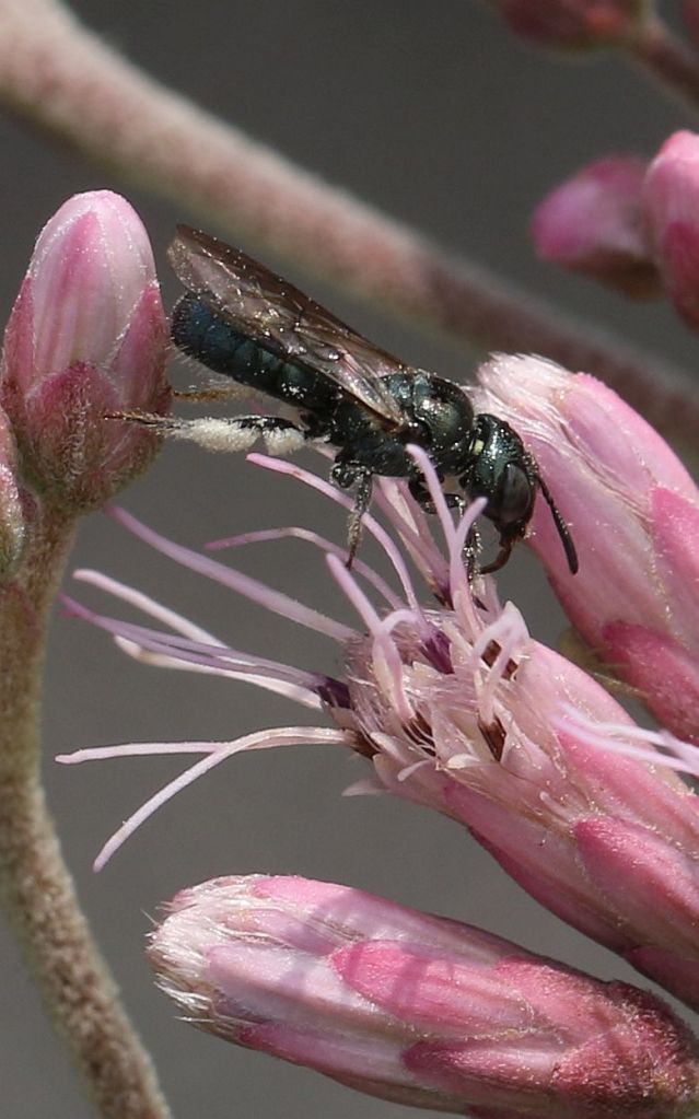
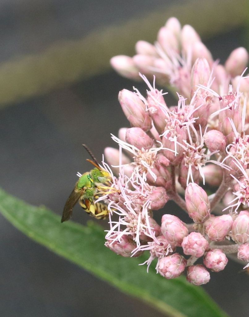
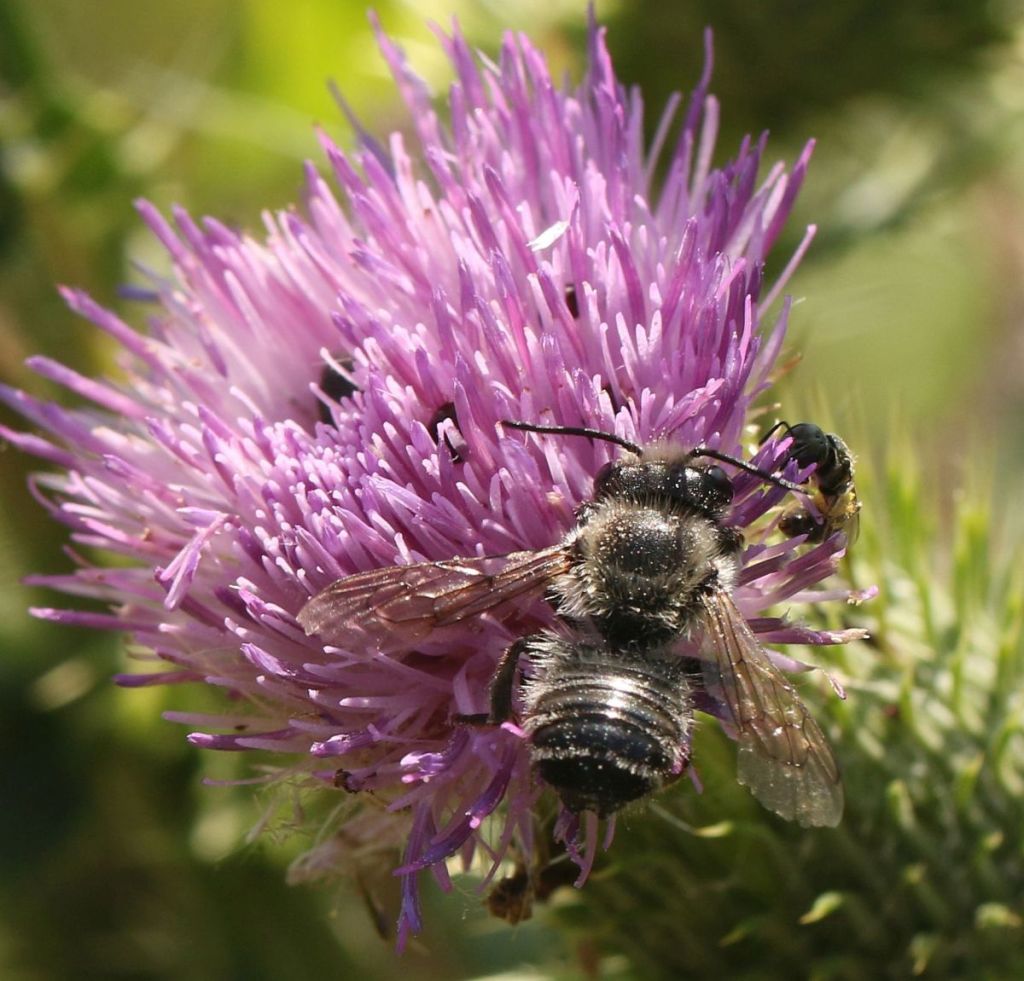
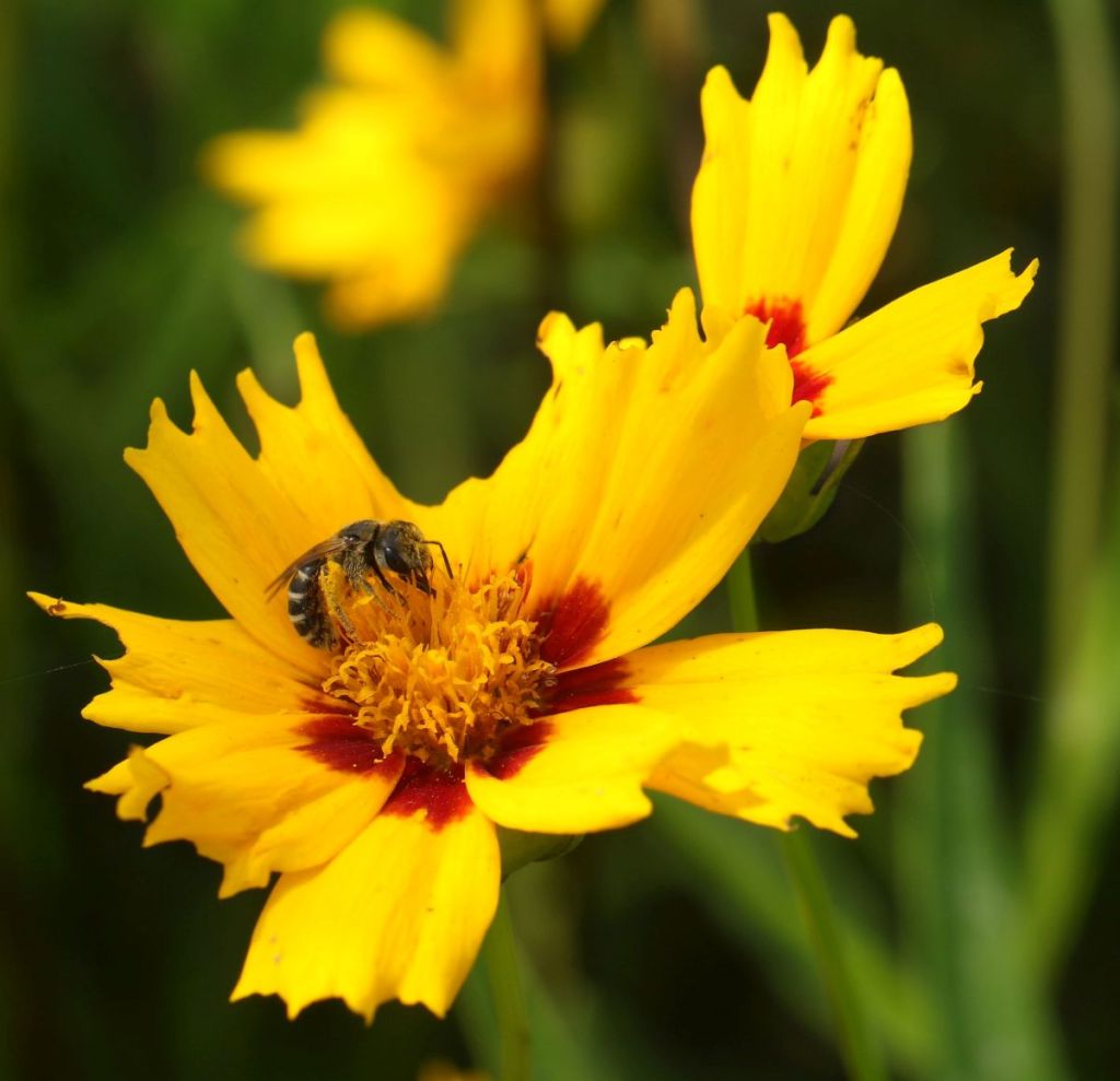
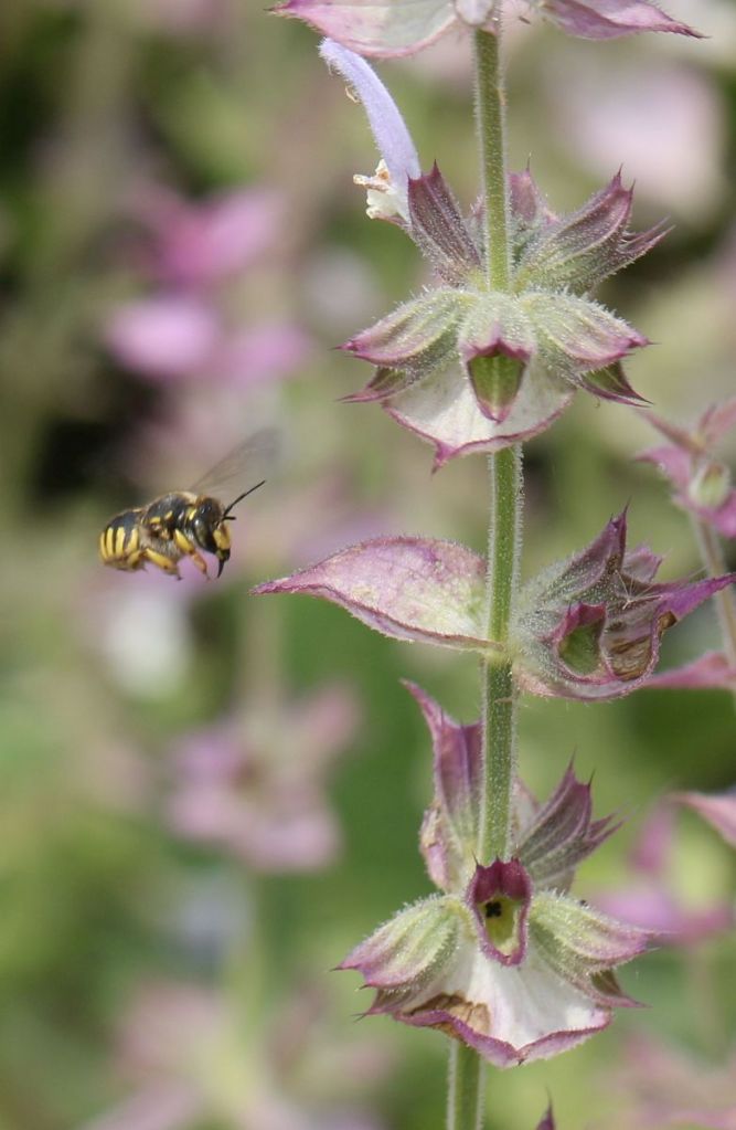
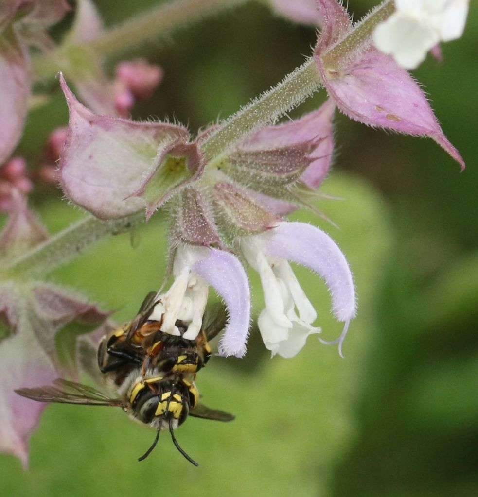
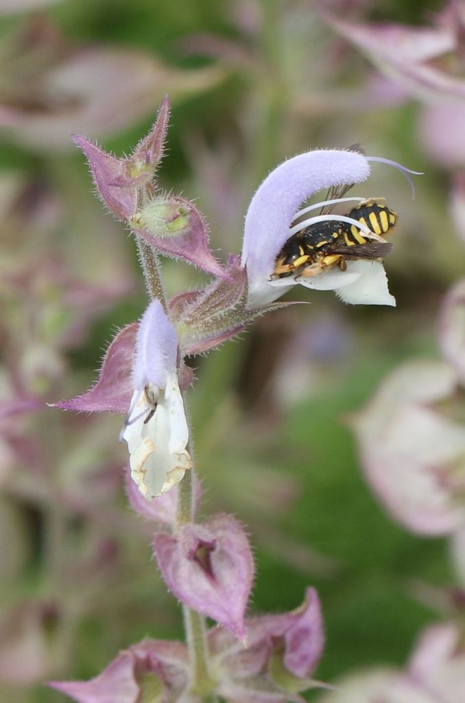
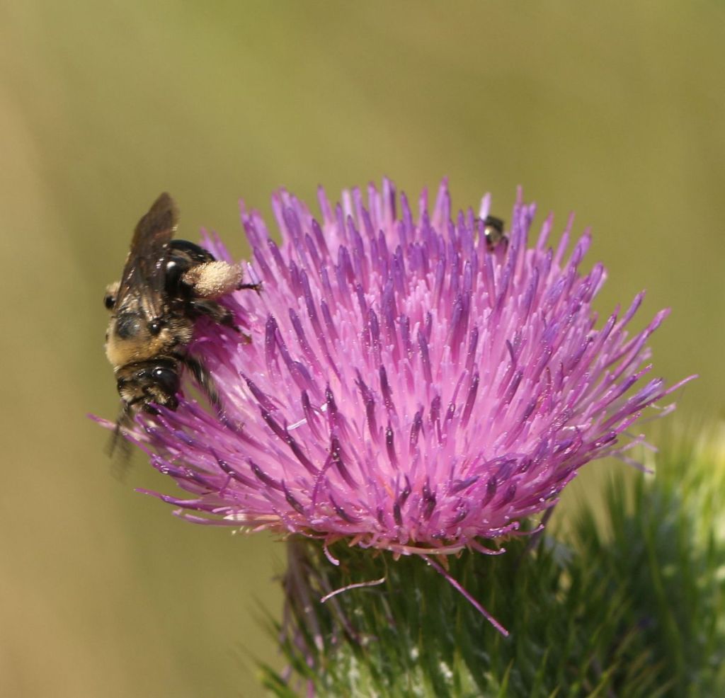
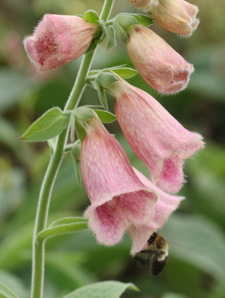
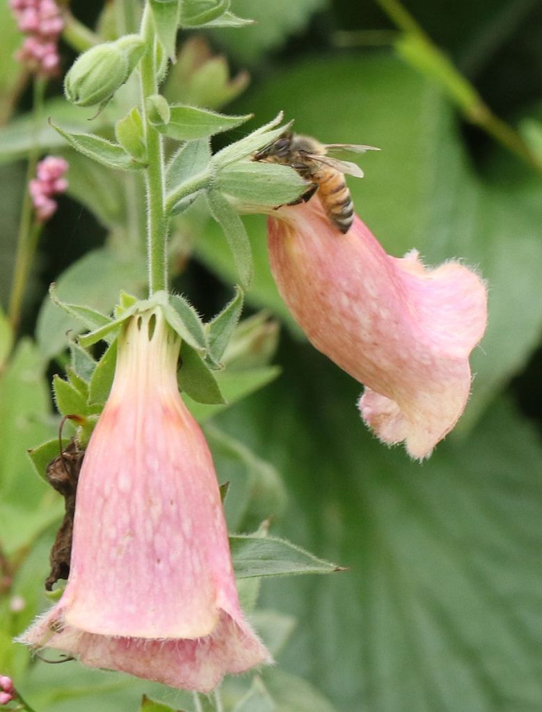
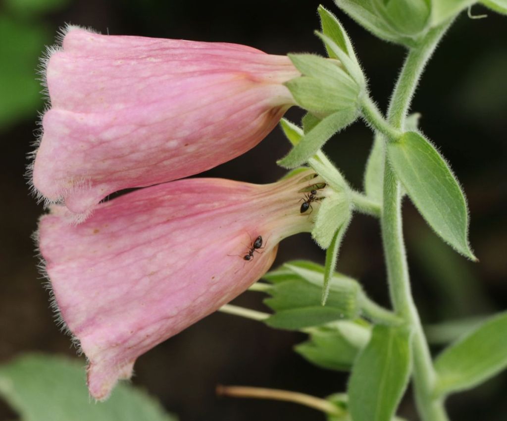
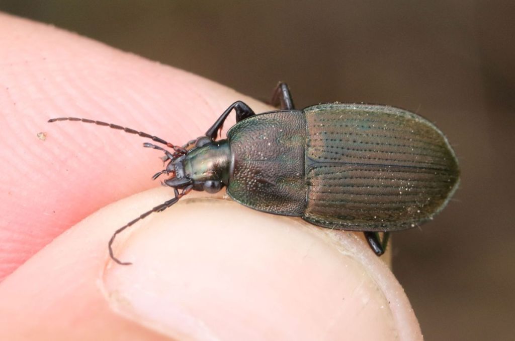
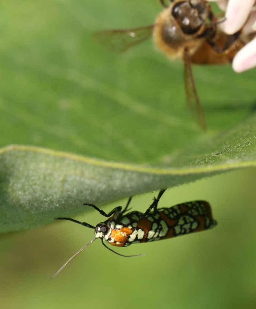
composite of different insect groups included

Figure 4. The six main insect groups tallied during this work, together with the name of the farm where the photos happened to come from.

Once the raw observational data were collected, they were corrected in two ways. First, the total number of sightings was divided by the duration of the observations to get sightings per minute of observation. This was necessary because, as noted earlier, not all observations lasted for five minutes. Next, the rate of observation on a given flower and for a given flower visitor (say, bumble bees visiting Zinnia at Little Seed Gardens on June 19^th) was divided by the average rate of observation for that insect taxon across all flowers observed at the farm on that date (i.e., all bumble bee observations on flowers at Little Seed Gardens on June 19^th). This was done because our goal was to calculate an index of relative flower favorability, and we wanted to take into account the fact that the ‘background’ levels of flower visitors might vary for a variety of reasons (e.g. if the preceding couple of days had been particularly cool and rainy, but the observation day was warm and sunny, then bumble bees might be especially active and so any ‘raw’ rates of observations from that day would likely over-value actual relative favorability).

The relative favorability ratings were then used in several different ways: first, they were used to create a table of favored flowers for each insect taxon; second, they were used to look for general patterns (e.g., were native vs non-native or cultivated vs wild-growing flowers more likely to attract certain taxa of insects?); and, finally, they were paired with Claudia’s species-specific flower abundance data for each survey unit in order to spatially and temporally map the appeal of a farm’s survey units for a given insect group.

RESULTS: What we found?

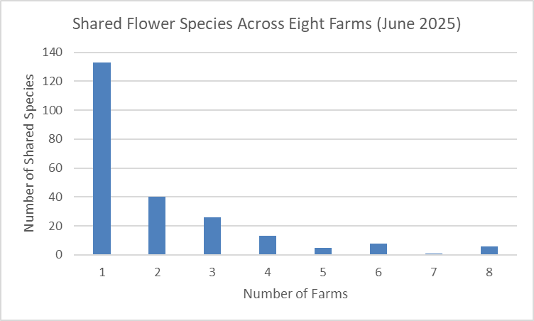
Flowers. We found a total of 371 species of plants in bloom across the nine farms (see here for the complete list). Of these, 162 were only found on a single farm (Figure 5). The farms ranged from harboring as few as three to as many as 37 unique blooming plants. Eleven species of flowers were found on all nine farms. These ubiquitous species were three native species: Daisy Fleabane, Horseweed, and Tall Goldenrod; and eight non-native species: Common Bedstraw, Common Ragweed, Common Yellow Wood-sorrel, Lady’s-thumb, Narrow-leaved Plantain, Red Clover, White Clover, and Wild Carrot (aka Queen Anne’s Lace). Farm-specific lists of plants observed in bloom are included in the individualized farm reports available from the links below.

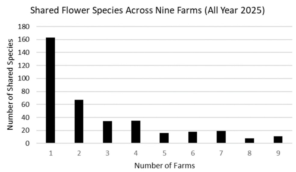
bar graph of the number of farms sharing the specified number of flower species

Figure 5. Graph illustrating the number of unique flower species (i.e., those found only at a single farm) in our study, as well as the number of species shared by two or more farms.

Not surprisingly, the size of the study area on each farm had a large influence on the total number of flower species tallied – in general, the larger the area we studied, the more different kinds of flowers we observed (Figure 6). It also didn’t come as a surprise that the larger cut flower farms (Hudson Valley Seed Co. and Treadlight) and the farm with intentionally installed and managed pollinator habitat (Hawthorne Valley Farm) had the highest flower diversity.

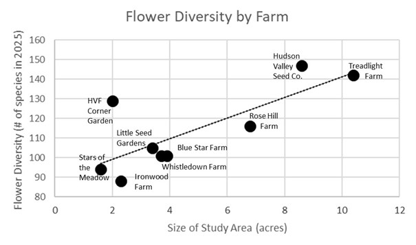
survey area size vs flower species richness

Figure 6. Flower diversity in relationship to the size of the study area at each farm

The following pie chart (Figure 7) illustrates the various categories of plant species observed in bloom at the nine farms in 2025.

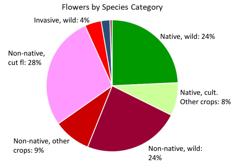
Figure 7. Plant species observed in bloom at the nine study farms by categories

Approximately 32% of these blooming species were native and about 52% were wild-growing.

For each farm, we created maps of flower diversity and abundance in each survey unit across the three sampling months (see example in Figure 8).

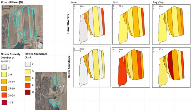
map graphics of flower diversity and abundance

Figure 8. Example of a map comparing flower diversity (upper row) and flower abundance (lower row) in the survey units of a farm. Maps for each farm are included in the farm reports linked to below.

In general, we learned that both flower diversity and abundance changed quite a bit in the survey units of each farm across the growing season. However, flower diversity and abundance were often not tightly correlated. Some survey units had a high abundance of the flowers of a few species. Others had a lot of species with few flowers each. Many were in-between.

The following graph (Figure 9) illustrates the distribution of flower species at the nine farms in four categories (wild-growing native species, wild-growing non-native species and taxa of uncertain native status, cultivated native species, and cultivated non-native species) across the survey periods.

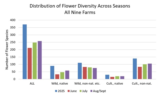
seasonal summary of the species diversity of various categories of flowers

Figure 9. Distribution of flower diversity by species categories across the survey periods. Wild-growing plants of unknown native status were included in the “wild, non-nat. etc.” category for simplicity. Farm-specific versions of this graph are presented in the individual farm reports.

Wild-growing native flowers and cultivated non-native flowers increased in diversity across the season, while the diversity of wild-growing non-native flowers was overall somewhat higher early in the season. There was some variation in these seasonal patterns between the farms (see individual farm reports linked below), but seven of the nine farms had a clear trend for increasing diversity of wild-growing, native species later in the season.

The next graph (Figure 10) shows the relationship between flower diversity (all species categories, across season) and management regime, based on the relative size of the total survey area (the sum of all survey units) in each management category.

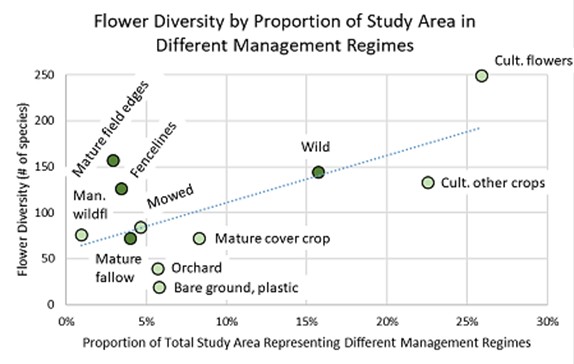
the flower diversity and size of different management regimes

Figure 10. Flower diversity in different management regimes relative to their portion of the total study area. dark green circles indicate unmanaged or lightly-managed habitats, the light green circles intensively-managed ones.

Of the unmanaged or lightly-managed habitats, mature field edges and fencelines had a disproportionately high diversity of flowers compared to the sample area they occupied, while wild areas and mature fallow each had a flower diversity that was expected for its proportion of the study area (their dots fell almost exactly on the trendline). This hints at the potential importance of narrow edge habitats. Not surprisingly, the beds of cultivated flowers were more diverse than expected relative to their size.

For each farm, we also created maps of the diversity of wild-growing vs. seeded/cultivated flowers in each survey unit across the three sampling months (for example, Figure 11).

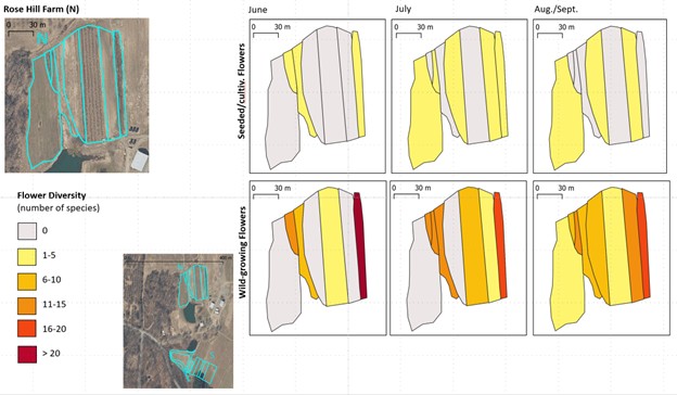
the mapped distribution of seeded and wild-growing flowers

Figure 11. Example of a map comparing the diversity of seeded/cultivated flowers (upper row) with that of wild-growing flowers (lower row) in the survey units of a farm. Farm-specific versions of this map are included in the individual farm reports linked to below.

These maps remind us of the fact that, even on farms with relatively high diversity of cultivated flowers, most survey units had significantly more wild-growing flowers. That was true not only for the fencelines and field margins, but also for more intensively-managed habitats.

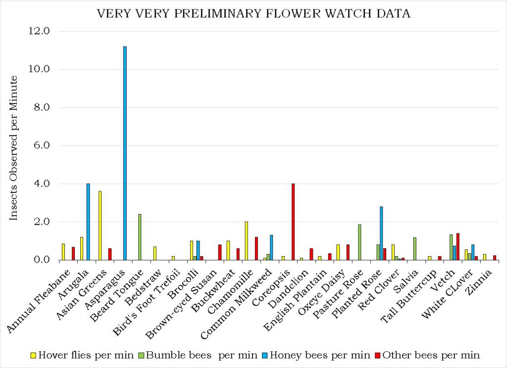
Species-level Flower Favorability. Table 1 shows the flower favorability ratings by insect taxon. As described in the “What did we do?” section, these were calculated by counting the bees (and other insects) seen during five minutes of continuously scanning new flowers of a focal plant species. For the given flower, all observation rates on all farms and during all outings were averaged.

Perhaps the most striking aspect of Table 1 is how distinct the lists are for the different taxa. Even amongst the different groups of bees, the repetition of favored flowers across the lists is modest. A few flowers, highlighted in color, were favored by three or more insect categories. These included: Appalachian Mountain Mint, Asian Greens, Bachelor Buttons, Common Milkweed, goldenrod, Ox-Eye Daisy, Smooth Blue Aster, Spotted Bee Balm, Viper’s Bugloss and Wild Bergamot. (Note that “goldenrod” refers to several species including Tall, Wrinkle-leaved and Smooth Goldenrods). One way of visualizing the roles of different flowers in supporting a range of flower visitors is by the use of radar graphs like those shown below (Figures 12 and 13 A-D).

Table 1. The flowers most favored by our six insect groups, based on observational data from all farms and all outings. Lists are alphabetical and only include those flowers with notably higher than average visitation rates by the given insect groups. Plant species native to the Hudson Valley are marked with an asterisk. Colored boxes highlight those species found on three or more lists. Black blocking indicates flowering times observed during the season. CLICK ON IMAGE FOR ENLARGEMENT.

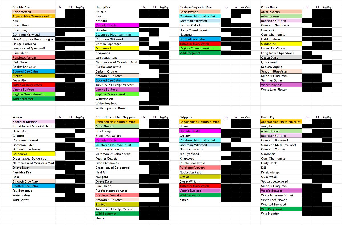
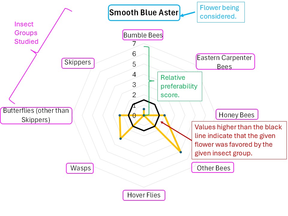
Table of favored flowers by insect group

explanation of a radar diagram used to show an insect groups flower preferences

Figure 12. Explanation of a radar diagram illustrating insect preferences for a particular flower. The names of the various insect groups studied is displayed around the circumference. The distance from the center point to the edge reflects the strength to which the respective insect group favored the particular flower by each insect group. The dark black circle indicates what would be a slightly above average favorability for that particular insect group across all flowers. Finally, the orange zig-zag indicates the data for the particular flower. In this case, Smooth Blue Aster was highly favored by ‘other bees’, and somewhat favored by wasps and Honey Bees.

Flowers with different offerings display different shapes on the radar graph, and scanning such images can quickly illustrate differences in the preferences associated with each flower. For example, in looking at Figure 13A, Common Milkweed’s wide-ranging appeal to larger insects (i.e., butterflies, bumble bees, carpenter bees and Honey Bees) is easily noted, as is the appeal of goldenrod (Fig. 13A), Sulphur Cinquefoil (Fig. 13B) and Bachelor’s Button (Fig. 13B) to the shorter-tongued creatures.

Even at this very general level, it is clear that this is, as mentioned, a case of “different strokes for different folks”. The variation in favored flowers amongst the insect groups relates in part to the mouth parts, color preferences, and nutrient requirements of the particular insects and, conversely, the flower depth, color, and pollen and nectar offering of the flower. For example, wasps do not usually have long tongues and so seem to prefer shallower flowers, such the goldenrods (Fig. 13A), the mountain mints (Fig. 13D), and Queen Anne’s Lace/Wild Carrot (Fig. 13D). Bumble Bees can usually tap deeper flowers, and so favor the likes of Wild Bergamot (Fig. 13A), Common Milkweed (Fig. 13A), and Viper’s Bugloss (Fig. 13A). However, long-tongued species can feed on shallow flowers, and shallow-tongued species can ‘short-circuit’ long flowers by biting through the tubes leading to the nectar reservoirs.

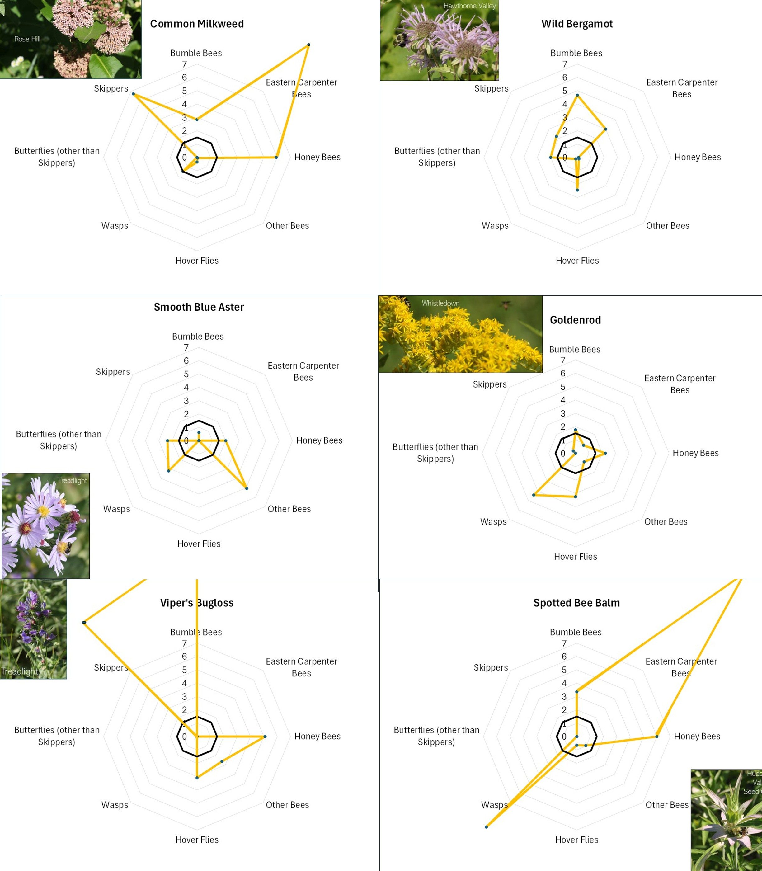
radar diagrams used to show various insect group's flower preferences

Figure 13A. Radar diagrams illustrating the favorability scores of various observed flowers. See Figure 12 for explanation.

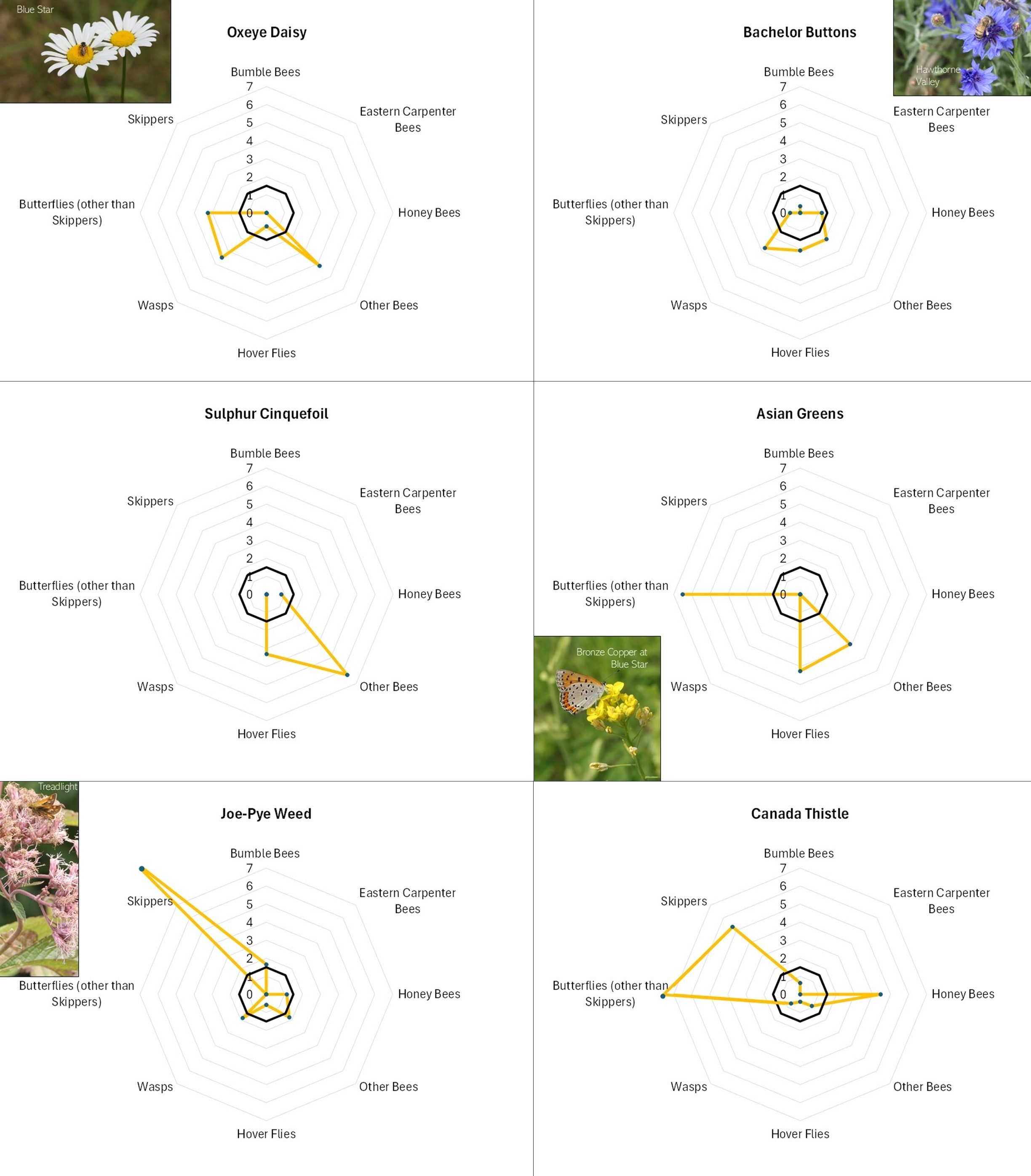
Figure 13B. Radar diagrams illustrating the favorability scores of various observed flowers. See Figure 12 for explanation.

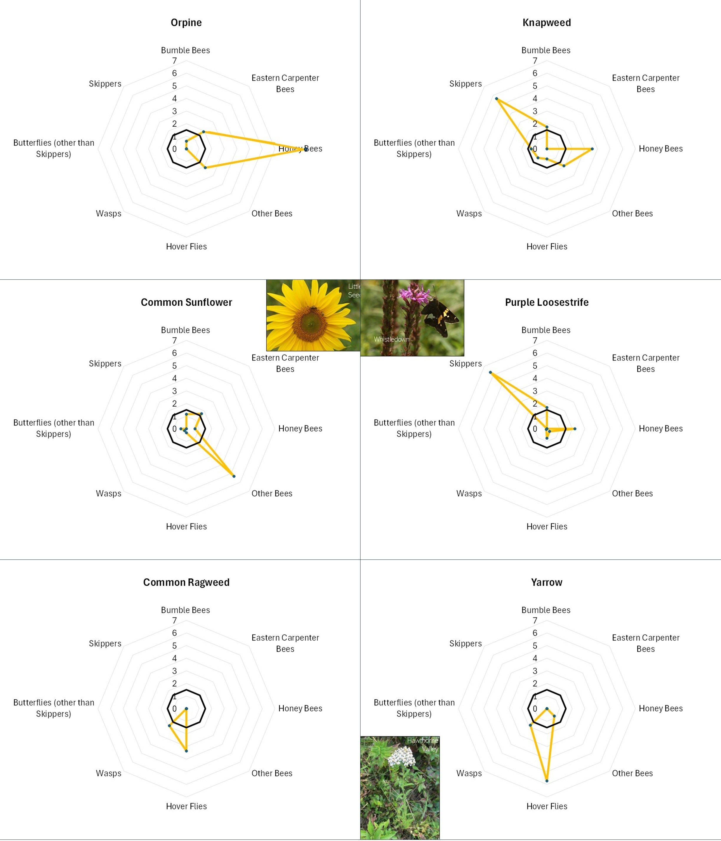
Figure 13C. Radar diagrams illustrating the favorability scores of various observed flowers. See Figure 12 for explanation.

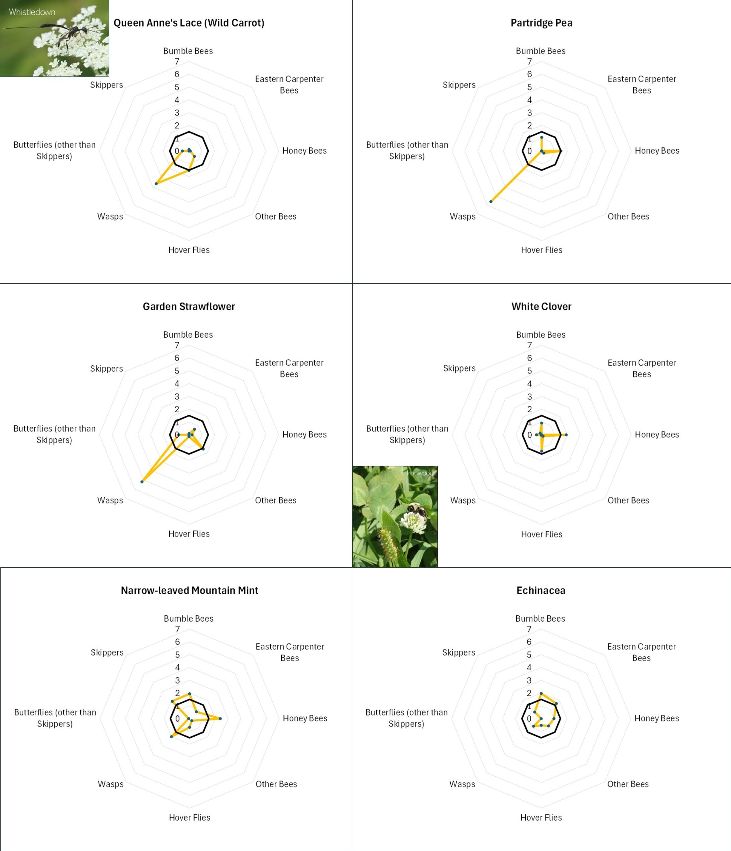
Figure 13D. Radar diagrams illustrating the favorability scores of various observed flowers. See Figure 12 for explanation.

A Couple of Key Questions. The above results pertain to specific flower species, but, as mentioned earlier, we were especially curious to know if any generalities could be made regarding the value to flower visitors of native vs. non-native flowers and of cultivated (seeded or planted) vs wild-growing flowers. To answer these questions, we compared the visitation rates of our focal insect groups to cultivated vs wild-growing and to native vs. non-native flowers (see Table 2).

Table 2. The average per-minute visitation rates of the different insect groups of seeded vs wild, and native vs non-native flowers.

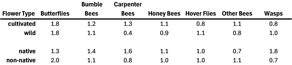
table showing insect visitation rates at native and nonnative and at seeded and wild-growing plants

In general, this seems to be another example of the ‘different strokes for different folks’ pattern. For example, some insect groups seemed to favor wild-growing plants and others favored cultivated ones. There may be a hint here that short-tongued creatures (e.g., wasps and hover flies) favor the wild flowers, perhaps because people are less likely to cultivate the small, shallow flowers these species can favor, and so such flowers are more common as ‘weeds’ (such as Queen Anne’s Lace/Wild Carrot or Daisy Fleabane). Butterflies and bumble bees seem noncommittal, while Carpenter Bees, Honey Bees and Other Bees seemed to favor the cultivated flowers. The Eastern Carpenter Bee’s apparently dramatic taste for cultivated flowers came about in large part because they favored a couple of the cultivated mountain mints, a couple of bee balms plus Nasturtiums and Celosia. However, Common Milkweed, a wild-growing species, was also frequented. Native plants were favored by those same Carpenter Bees (because they used several native but cultivated species), but also by bumble bees and wasps, while butterflies and other bees seemed to favor the non-native flowers. Note in relation to butterflies that we are ONLY talking about nectaring by adult butterflies, it’s likely that caterpillars are more discerning and that native butterfly species would favor native host plants as larval food.

Based on the limited evidence from our work, we would say that both cultivated and wild-growing, and both native and non-native species have roles to play in supporting our flower visitors.

We’ll return to the management implications of these results after describing the content of the individualized farm reports.

MAPPING: Individualized Farm Reports

Overview. While the above general information is useful, farm-specific maps showing the occurrence of plants, the management regime, and apparent favorability of survey units for flower-visitors can provide an intuitive and useful outline of each farm’s flower resources. Thus, many of the data generally described above were mapped for each farm. These maps are included in the farm reports available as links below. In the spirit of discussion that motivates this group, those individual farm results are being made available to all. Nobody is doing things ‘better’ or ‘worse’ than anybody else, but each farm is different and so can provide new lessons.

The links immediately below will take you to .pdfs of each farm’s report:

Blue Star Farm Report

Hawthorne Valley Farm Report

Hudson Valley Seed Co. Report

Ironwood Farm Report

Little Seed Gardens Report

Rose Hill Farm Report

Stars of the Meadow Report

Treadlight Farm Report

Whistle Down Farm Report

Following, we illustrate what you can expect in the individual farm reports with examples from Rose Hill Farm.

Survey units and Management Regimes. The first step was to outline the area that would be studied on each farm, to delineate survey units, and to determine their management regimes. As noted earlier, due to practicality, in all cases the potential foraging range of a bee substantially exceeded the study area we surveyed, and they may well be collecting resources farther afield. Work we did on several Hudson Valley orchards suggested that land use within at least 1600 ft of the orchard affected the bees found during spring bloom, indicating a relatively wide ‘sphere of influence’.

Rose Hill happened to be unique in that we decided to study two completely separate sections of the farm. Figure 14 shows the survey units we delineated in the two study sections in July. On some farms, the shape or the number of survey units varied somewhat across outings. This could occur if, for example, a field with several beds of different crops early in the summer (which would be divided into several survey units) were to be plowed up and made into one uniform field with a cover crop (which would then be delineated as a single survey unit) later in the year.

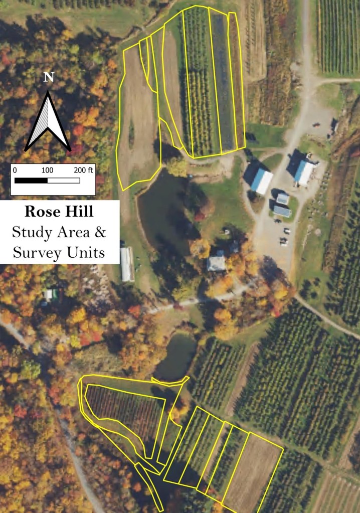
aerial showing survey units at Rose Hill

Figure 14. Study area and survey units delineated at Rose Hill during July.

The survey units usually represented several different management regimes. For example, at Rose Hill (Fig. 15), the survey units represented fruit crop production (orchard and blueberries), mowed lawn, cultivated flowers, fenceline, mature cover crop, mature field edge, and wilder areas. On each farm, an effort was made to include examples of both more and less intensively managed habitats, because of our goal to compare the value of wild-growing and cultivated flowers.

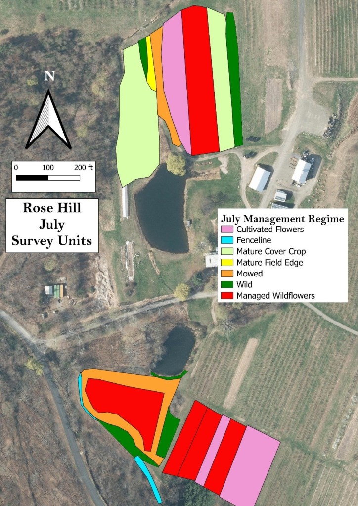
map showing management regimes at Rose Hill Farm.

Figure 15. Generalized management regimes in the Rose Hill survey units during July.

Botanical Mapping. As described above, within each of the survey units, the flowering species (and only those species actually in bloom during the given outing) were recorded three times during the 2025 season, and their individual and total flower abundances ranked. While it would be theoretically possible to do, we have not mapped the occurrences of individual flower species. Instead, we mapped summary statistics such as flower abundance and flower diversity, and the ratio of wild-growing vs. cultivated flowers (see example maps above).

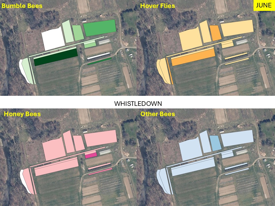
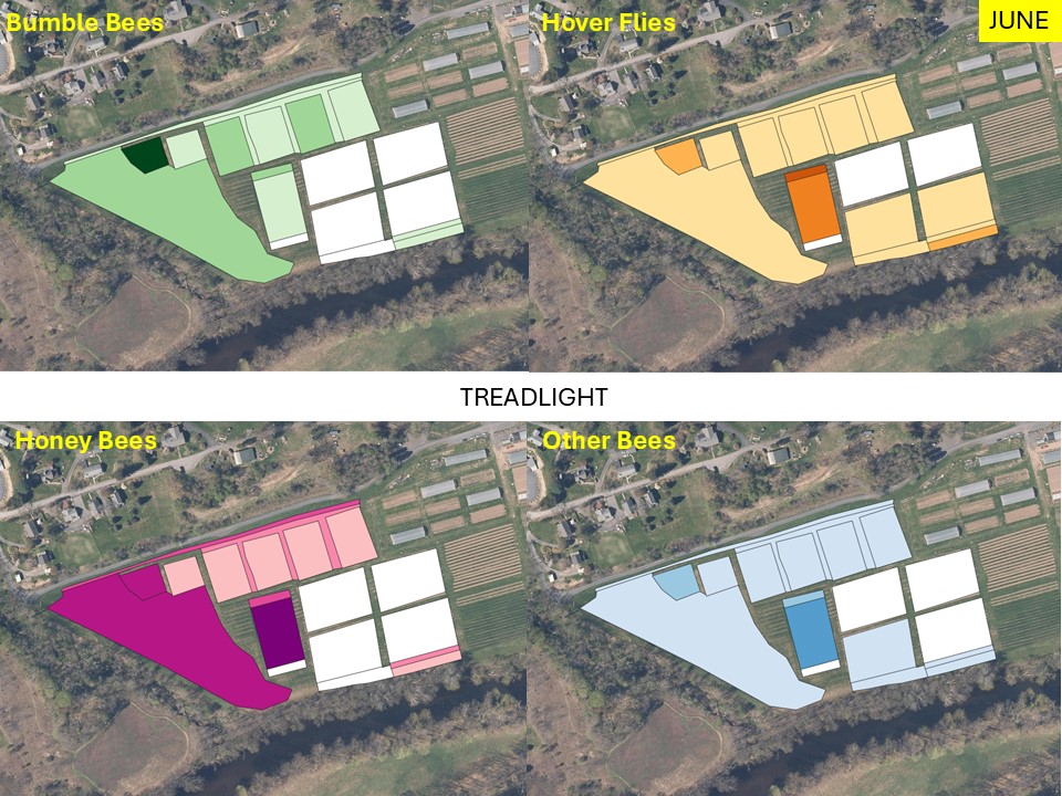
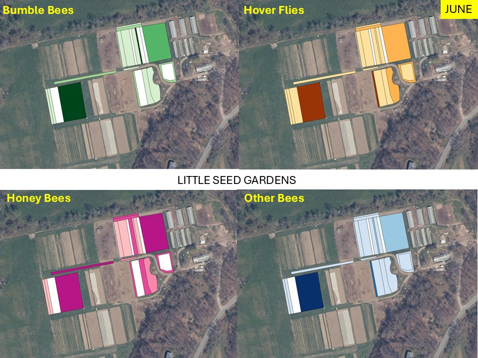
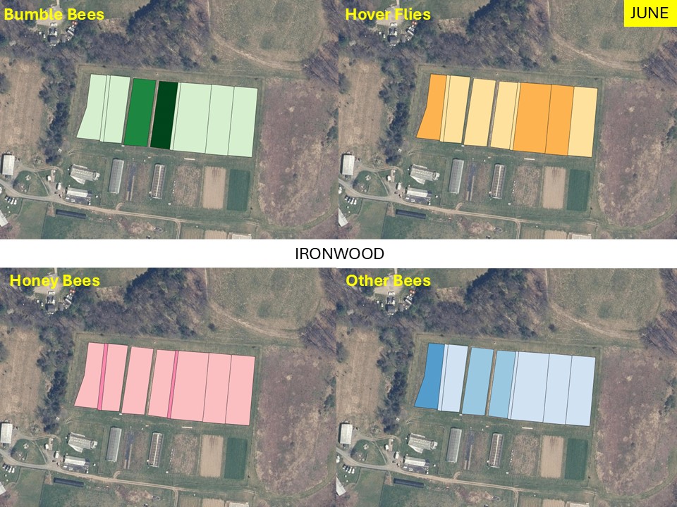
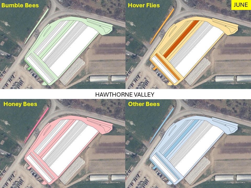
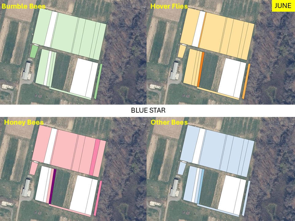
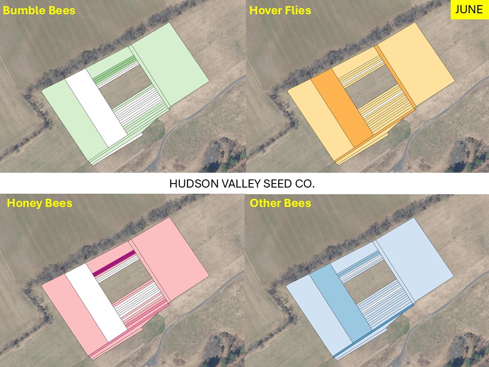
Mapping Flower Favorability. Finally, we took the flower information and combined that with insect-taxon specific flower-favorability ratings to create predicted favorability ratings for each survey unit and insect taxon during each of the three surveys. (Figures 16 A-F). Within insect groups, it is valid to compare colors across outings and farms. In other words, were one looking at bumble bees, a yellow bed at Rose Hill in July is indeed predicted to be more favored than a bed that is blue at Whistle Down in June. However, in absolute terms, colors are not equivalent across insect groups, even within the same farm.

Remember, these maps are NOT maps of actual insect densities. Such maps would be interesting but were beyond our means this past summer. Instead, these maps show the predicted favorability of each survey unit for a given flower visitor based on, as already noted, the unit’s botanical composition and the observed flower visitation rates gathered across all farms and survey months. Nonetheless, we think they provide a relevant depiction of the flower resources on offer.

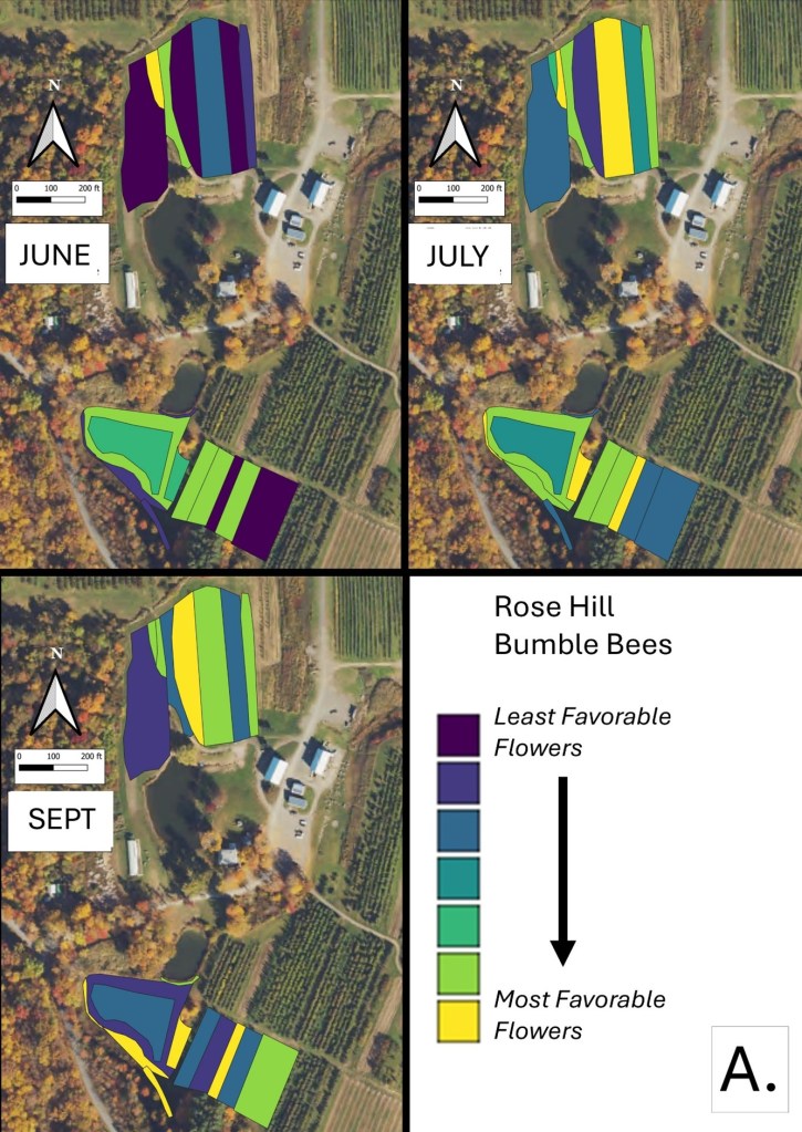
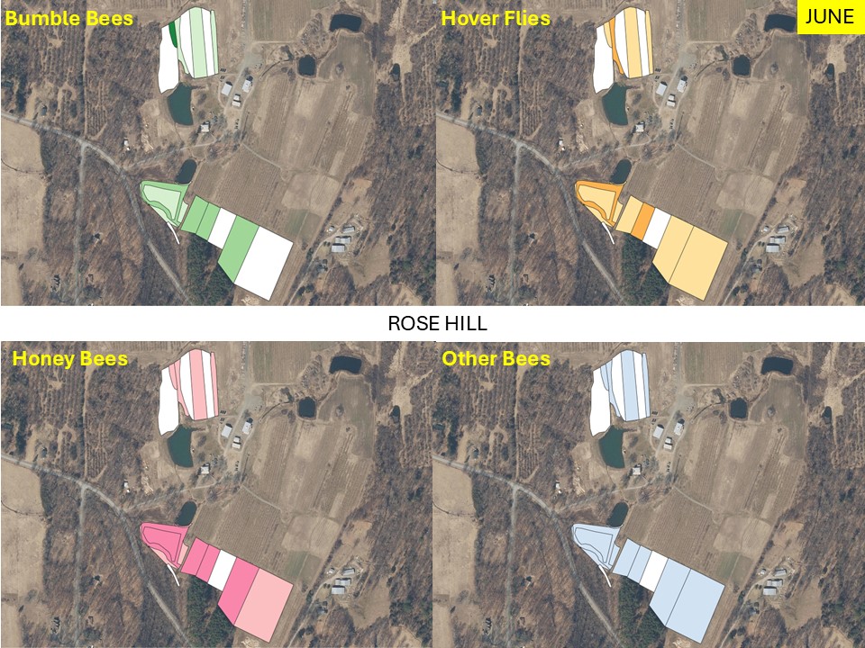
a map of flower favorability for bumble bees

Figure 16A. Flower favorability for bumble bees in the different survey units and months at Rose Hill. Generally, darker signifies less favored flowers, and lighter colors mean more favored.

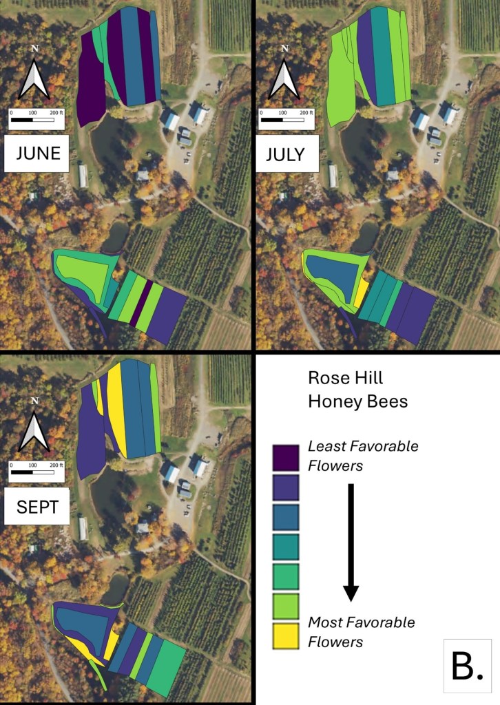
a map of flower favorability for Honey Bees

Figure 16B. Flower favorability for Honey Bees in the different survey units and months at Rose Hill. Generally, darker signifies less favored flowers, and lighter colors mean more favored.

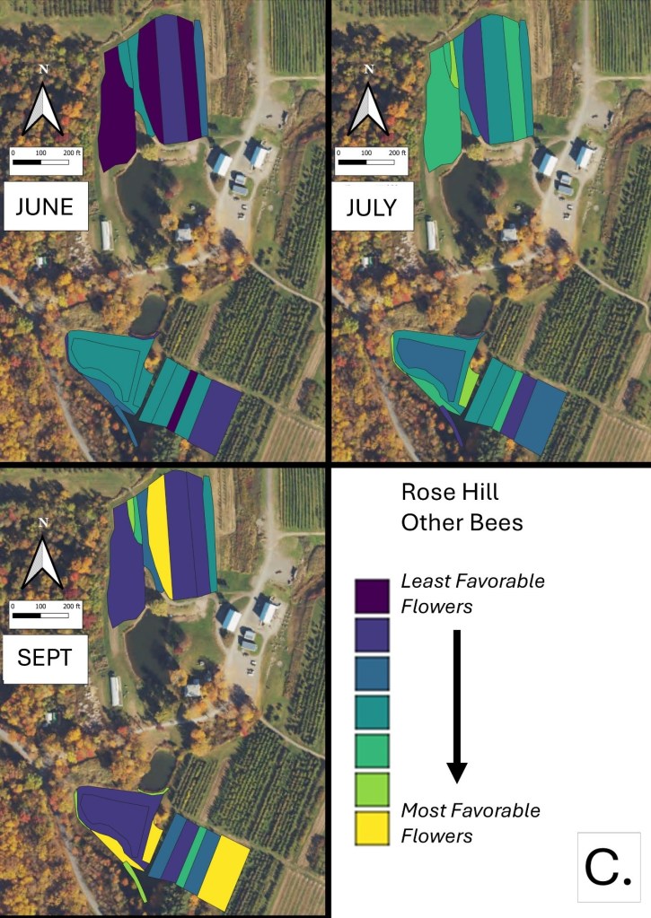
a map of flower favorability for 'other bees'

Figure 16C. Flower favorability for ‘other bees’ in the different survey units and months at Rose Hill. Generally, darker signifies less favored flowers, and lighter colors mean more favored.

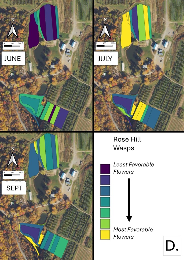
Figure 16D. Flower favorability for wasps in the different survey units and months at Rose Hill. Generally, darker signifies less favored flowers, and lighter colors mean more favored.

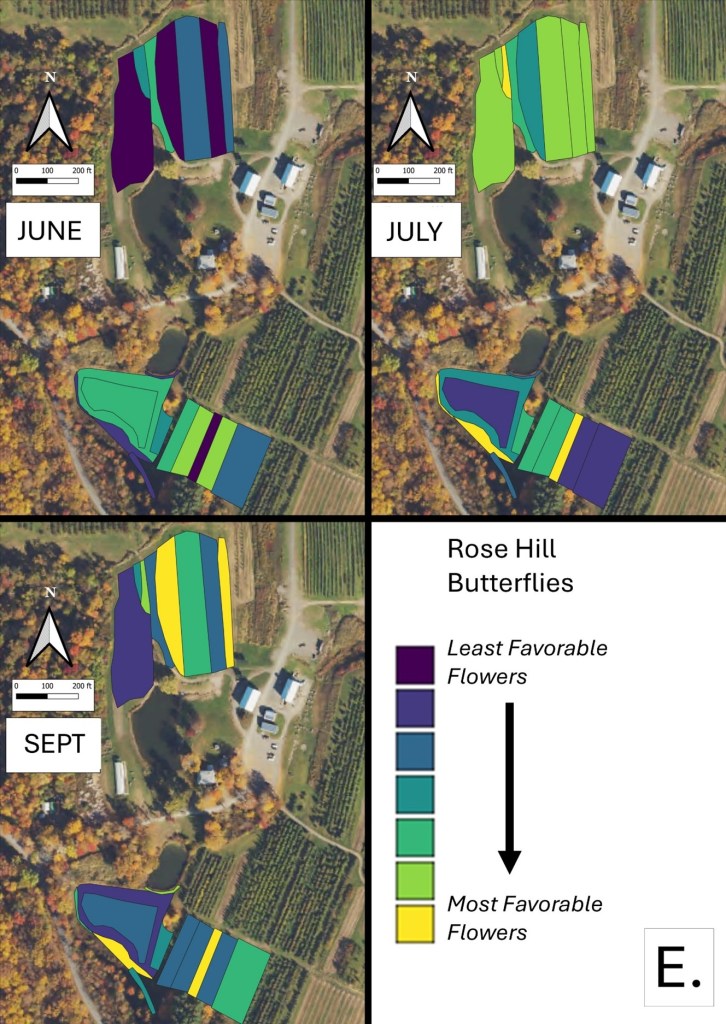
a map of flower favorability for butterflies

Figure 16E. Flower favorability for butterflies in the different survey units and months at Rose Hill. Generally, darker signifies less favored flowers, and lighter colors mean more favored.

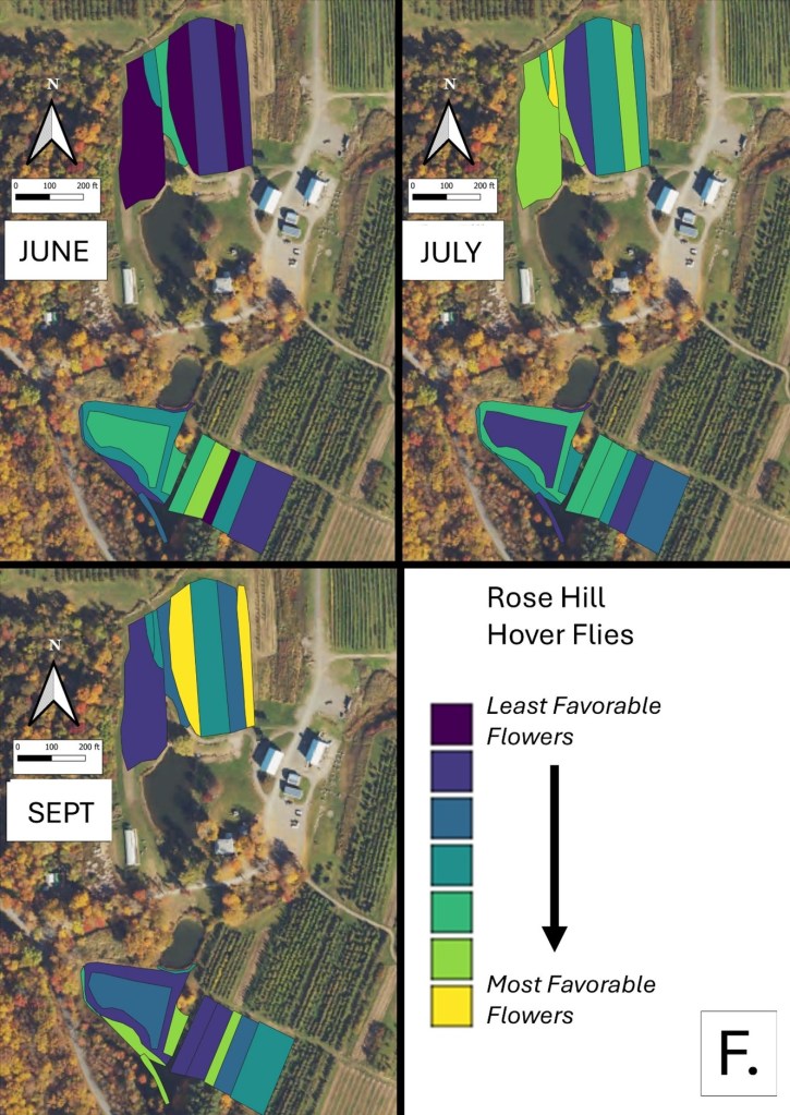
a map of flower favorability for hover flies

Figure 16F. Flower favorability for hover flies in the different survey units and months at Rose Hill. Generally, darker signifies less favored flowers, and lighter colors mean more favored.

SO WHAT?: How to use these data

Table 1 (the table of favored flowers by insect taxon) can be useful because it provides broad-brush information on what flowers might support which flower visitors. This information is hardly unique (see for example the work of Xerces), but it is specific to the insects and plants of our region. If, for example, you wanted to create flower beds that offered resources to an array of insects, you could plant (or allow to bloom) a mix of flowers from across the lists for each taxon. Alternatively, if you wanted to focus on attracting/supporting one particular insect group, then you could plant heavily from that taxon’s flower list. Furthermore, you could somewhat refine what seasons you wanted to emphasize – if the maps suggested low bumble bee flower resources in June, then you could look for June-flowering, bumble-bee favored flowers. Do note that only flowers actually observed at our study farms during the summer 2025 were considered for inclusion on this list (see here for the complete list of all flower species observed during this study); there are surely other flower species, not seen during our study, that can support these insects.

The potential use for the favorability maps will also depend on your goals.

In glancing over the maps (Figures 16 A-F), first train your eyes – dark blue means low predicted favorability while bright yellow means higher favorability. So, if you scroll through the maps below, which insect groups seem to be most/least favored by the flowers at Rose Hill? In other words, which maps are lightest and darkest overall? My eye suggests that bumble bees are relatively favored, while hover flies, for example, are not. Whether that observation prompts management considerations depends, in part, on the importance attached to the aphid-controlling habits of many hover fly larvae. Were one interested in augmenting hover fly resources, one might consider planting more of the flowers listed in the hover fly column of Table 1. Do you see anything surprising? For example, you may well have correctly predicted that your bed of cultivated flowers would be attractive to Honey Bees and bumble bees, but did you realize that, for example, ‘weeds’ in your crops were supporting aphid-eating hover flies or that the taller vegetation along your fence was favored by wasps? If either of those are desirable, then how might those resources be expanded?

The next thing one can do is inspect the three monthly maps on each insect group’s page and ask, ‘how good does across-the-season flower favorability seem to be?’ While some insects do fly for only a relatively short period of time and so only need flower resources for that limited period, many others fly throughout the season and need good resources across that period for their populations to flourish. Look, for example, at the ‘other bees’ maps in Figure 16C. Note that favored flower resources for ‘other bees’ seem to be relatively sparse in June and July, although the situation looks better come late summer. Were one interested in promoting populations of ‘other bees’, then one might again refer to Table 1, and now search for early flowering species that are favored by ‘other bees’. Indeed, broadly speaking the availability of favored flowers in June looks to be low for most insect groups at our example farm (Rose Hill; Figures 16 A-F), and this observation might encourage the planting of a range of early-flowering species. (Realize that there is more to life than June-September, but we did not collect data on it. Expanding our surveys to include earlier in spring might be one important future undertaking.)

Finally, one can scan the maps and ask if there are any survey units which are consistently low in their favorable flower offering and, at the same time, are not integral to crop production. One potential example at Rose Hill was the westernmost unit of the northern study area. It was in ‘mature cover crop’ in mid July and, other than supporting a relatively high density of wasp-favorable flowers during that month, it seemed to provide relatively few floral resources. Of course, it may well be that that field is in rotation for some future use and not really available for tweaking, but, if not, then it might be a space where flower seeding could increase its contribution to supporting flower visitors.

We realize that there are numerous other considerations that come into play when planning flower management (e.g., reducing potential tick contact or Groundhog habitat, or increasing the ease of farm operations). These maps are only a resource that, if so desired, can be one ingredient contributing to your overall management decisions. More specific thoughts are provided with each farm report.

MANAGEMENT CONSIDERATIONS: Questions raised and potential actions.

In considering the above flower favorability maps, we have walked you through some examples of specific management considerations. The linked farm reports include additional thoughts specific to each farm. However, in preparing those reports and considering those results, certain general management considerations and questions came to the fore.

One key consideration is that, as mentioned earlier, our study areas were generally much smaller than the home ranges of any of these insects. That meant that what we were observing in our survey units reflected not only the conditions in those units, but also the conditions – flower abundances, nesting resources, pesticide applications etc. – in a much larger area. Management for on-farm flower visitors is a bit like life: you do the best you can with what you’ve got, but you also realize that ‘outside forces’ will also play a substantial role. While we cannot hope to identify and quantify all the ‘outside forces’ affecting on-farm flower visitors, it may be worth considering, and to some extent exploring, the availability of shoulder season flowers outside and inside the study area, soil texture in relationship to ground-nesting bees and wasps, and additional flower resources during the main survey period but outside the survey area. We did not, but we could, try to document the role of, for example, forest or wetland areas in providing flower resources and potentially nesting resources. Other factors relating to, for example, climate change and off-farm land management (e.g., urbanization, use of pesticides) might help put on-farm results in context, but may not be as interesting because they are largely outside a given farmer’s management purview.

There is however at least one aspect of the larger landscape management that might be worth exploring further and that is the potential for synergies between collaborating, adjacent farms. Out of the nine farms we studied last summer, at least three were adjacent to other ‘ecological’ farming operations. In one case, this was a focal veggie farm next to a flower farm and, in two cases, it was focal flower farms adjacent to another operations. What benefits and costs derive from such juxtaposition? In terms of encouraging a broader consideration of what is meant by an ‘agrarian landscape’, might it be useful to try to document these interactions in greater depth?

More broadly this work posed at least a quartet of general agroecological questions:

To what degree do ample flower resources augment pollination services by increasing pollinator populations and to what degree do they reduce crop pollination by distracting pollinators from that task? Others have studied this somewhat in relationship to fruit pollination where a sudden, short burst of flowers calls for an ‘all hands on deck’ response from pollinators. How does this same logic apply to flower beds amongst ‘pollinator hungry’ crops? Trying to provide a detailed dynamic heat map of flower visitor abundances across the season at even a single farm might help illustrate the ebbs and flows of pollinators and other insects, which, in turn, might help us better incorporate these movements into the pollination of crops. Such a consideration is less directly relevant to parasitoid wasps and hover flies, where the main agroecological service is not directly provided by the flower-visiting adult, but rather by the feeding of the larvae (either as parasitoids or aphid-eating maggots).

And, related to that and the earlier considerations, what are the limiting factors affecting flower-visitor populations? Think of a football team and what affects its chance of winning – if the quarterback can’t throw worth a darn, then that may be the most immediate limit on the team’s chance of success, but once you get an all-star quarterback, then the shoddy defensive team might be the main limit, get them up to snuff and your running back’s slowness might be the sticking point… Likewise, if flower visitors are receiving all the flower resources they need, then nesting resources, host availability (in the case of parasitoids), hibernation sites etc. can all become important. Our work did not indicate a strong one-to-one relationship between flower favorability and flower-visitor numbers. While this might, legitimately, bring our methods somewhat into question, it might also suggest the presence of other limiting factors whose identification might be an important contribution to facilitating management. Ways of exploring this might include augmenting nesting resources (e.g., bee hotels and sand piles for ground nesters) and seeing how much interest there is from the insect community – ample and rapid adoption of such resources might suggest they have, indeed, been limiting.

How relevant is ecological lag time? Insect populations cannot respond instantaneously to increased flower resources. Our work at Ironwood and at the Farm Hub suggest that part of what is important is what butterfly biologist Ann Swengel calls ‘consistent diversity’, that is a diversity (and abundance) of resources that persists across time. The long-term aspect is what gives insects the chance to ‘settle in and raise a family’ (or, better put, to raise families across multiple generations). In thinking about farm management, this doesn’t mean that the same flowers have to be found in the same beds year after year, but rather that the same suite of flowers, indeed same suite of habitats, needs to be found somewhere on the farm across multiple years if one is hoping to support higher/more diverse insect populations in the long run.

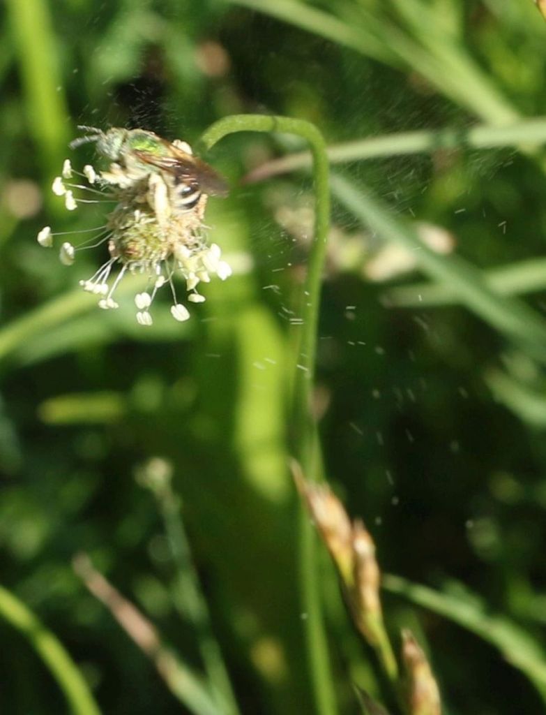
How important are ‘native’ and wild plants? The work reported here suggests that the different flower visitors do show distinct flower preferences, but that native vs. non-native or cultivated vs wild are not necessarily the sole, and perhaps not even the primary, determinants of those preferences. It appears that, within the very limited context of our work, both native and non-native (and cultivated and wild) flowers can make positive contributions. HOWEVER, nativeness is likely important in ways that we barely scratched with our methodology. For example, while many moths and butterflies might be relatively loose in the flowers they choose to nectar from, their leaf-eating larvae are often much more picky and native insect species are likely to favor native host plants for their young (although they sometimes grow to like naturalized non-natives too). Further, while the bee groups we studied did not, as a whole, show an overwhelming preference for native flowers, there are rare, specialized bees whose life histories are indeed closely tied to native plants. The Macropis bee we documented feeding on Fringed Loosestrife (Lysimachia ciliata) is one such example. In sum, were you able to raise only native flowers, your contribution to insect conservation would likely be higher, but non-native flowers can also make a positive contribution so long as their limitations are understood.

If we agree that augmenting the availability and diversity of favorable flowers is one (but not the only) useful way of contributing to flower-visitor abundance and diversity, then we suggest the following framework when thinking about potential “tweaks” to farm management in order to increase flower resources:

Vibrant fencelines – How close to the fence do you need to keep things mowed and at what frequency? How to keep vines and/or invasive shrubs from overwhelming the fencelines while mowing less? Note that ‘looser’ management might not only increase flower abundance and diversity, but also expand nesting sites for those insect species seeking hollow plant stems or thatched areas for their nests. Depending on the specific situation of the farm, looser management of fencelines might however also invite the spread of invasive plants and the establishment of vegetable-raiding Groundhog colonies.
Enrichment seeding/planting in wild areas – Several of the study farms had loosely-managed oldfields, wet meadows, or shrubby areas which, although they did provide some flower resources during a part of the growing season, have the potential to provide flowers over a longer period and/or to support more diverse and/or abundant flowers. Short of a complete conversion, which might be expensive and not even be desirable if the area already does contain good patches of flowers, one could consider tilling up small areas and seeding or planting them with desired flower species.
Dedicated annual or perennial flower beds within the cropped area – These areas may also improve nesting/hibernation habitat (e.g., “beetle banks”), but be forewarned, such habitat can also host Groundhogs and voles!
Reduced mowing frequency/changed timing/increased mowing height of lawns – What is the goal of the lawn mowing and how might those goals be met while at the same time providing more room for flowers?
Reduced mowing frequency/times of lightly managed areas, such as mature field edges, old fields, wet meadows – As with fencelines, looser management can also enhance nesting/hibernation resources for insects, but potentially also facilitate invasive plants and Groundhogs.
Welcoming the weeds – Of course, there are good reasons why this sometimes conflicts with food production, but when possible being tolerant of (or, at least, feeling less guilty about) in-bed flowering weeds might be appropriate given the how attractive some of the ‘weeds’ seemed to be for certain flower visitors.
Editing hedgerows and margins for flowering (native?) shrubs – Hedgerow installations, while potentially valuable, can be daunting. However, the removal of less desired woody plants can provide more growing space for those you do want. While we did not include many woody plants in our surveys last year – in part because we only started them in June when most woody plants are done flowering – we know from the literature that some of them provide important early-season flower resources and could include them in expanded future surveys.

CONCLUSIONS: What are our last thoughts and yours?

These analyses have, in some ways, been a ‘proof of concept’. We can take field observations of flowers and flower visitors and convert them into farm-specific maps, but if the results seem esoteric and not useful, then it has been a wasted effort.

The most pressing conclusion is thus a question: is this sort of information useful to you? If not, then further exploration of this theme makes little sense.

However, if it does seem useful, then how could it be made more useful? Gathering more flower-visitor observations in order to refine our assessment of flower favorability might be worthwhile. No doubt some of our results are flukes caused by having relatively little data (for example, Viper’s Bugloss seems to be a winner, but we only observed it on one farm on one date). More observations, potentially from more farms, could help us understand how generally applicable our results are.

We could also refine our visual bee, wasp, and hover fly identifications. Although species-level identification may only rarely be practical, greater refinement is possible. Indeed, as the summer wore on, aided by learning eyes and diligent photography, we were able to gather somewhat more detailed ID information. From an applied perspective, such information may have only limited value unless it reveals certain closely knit relationships between, say, a bee and the pollination of a certain flower or a particular wasp who attacks a particular host. However, from the perspective of biodiversity conservation such IDs can be crucial, because it is only at this level that we will truly understand when a given farm or flower is supporting rare species.

We could also expend more effort trying to refine our understanding of the correspondence between flowers and flower visitors by looking at more flower beds on more days or at more times of day. This immediately raises practicality issues unless you want a live-in biologist on your farm. While extensive sampling might not be feasible or even desirable, we have recently collaborated with Laura Figueroa of UMass Amherst to use sound recordings to assess bee presence. This technique has the potential to give us a much more refined picture of bee use by allowing us to assess bee presence on multiple days at multiple times. Such an approach might also help us test our maps by giving us bee activity data in each survey unit (recall that our flower visitor observations were tied to flower types, not survey units) and even in wilder areas, such as adjacent forests (might we, for example, be able to document what habitats are most sought after by nesting bumble bees?).

Reviewing the data at hand, a central conclusion that we have already re-iterated several times is the idea of ‘different strokes for different folks’, that is different flower species and different flower classes (i.e., cultivated vs wild-growing, native vs non-native) are attractive to different groups of insects. These are results which could be refined if, as mentioned above, we are able to improve our visual identification of flower visitors. However, even at this general level, we hope that this conclusion helps emphasize the value of on-farm botanical diversity not only in a single year, but also across years – as some of our work has suggested, insect populations cannot instantaneously react to enhanced resources. On-farm botanical diversity is the groundwork that will support on-farm entomological diversity, which, in turn, could supply a greater diversity of agroecological services and add contribute to regional insect conservation in the region.

Posted on December 22, 2025December 22, 2025 in farms, insects, plants

A Farmer-Ecologist Research Circle Description and links to Materials about Some of this Summer’s Work

A Preamble (or was that ‘Pre-ramble’?) of Sorts.

It can be useful to periodically restate what it is we’re trying to do. The following are a few words that were shared at the 17 Dec. 2025 meeting of the Research Circle. In part, they’re meant to help newcomers understand what we’re up to and to answers some questions we have received.

The Research Circle is not the project of any one person or organization. While we are fortunate to get funding from the Farm Hub and the Circle includes staff from Hawthorne Valley, it really derives from a shared desire to work together on topics of mutual interest. Some of us have been at this (on-farm ecological research, farming) for a while, and we are searching for ways to build a community of like-minded individuals to design, execute and act upon ecological research of the community’s own design.
That means that the Circle has no other existence than all of you, all of us. It exists for as long as we want it to and in the shape we choose for it. It is very much a work in progress. Some of us have tried to establish an initial framework in order to get it off the ground but this is intended as a starting point, not an end point.
Reflecting on our own strengths and weaknesses, we as the ecologist did establish one set of boundaries on our own work: There are many, many relevant research questions around farming. We cannot hope to answer them all, nor do we have the capacity to do so. While, to a certain degree, we can bring in the expertise of others, for now what we can offer as researchers is a focus on the role of on-farm habitats in supporting nature for its own sake and for its interaction with production.
In this context, the reports presented in the Fall are the research feedback from projects we all designed together the previous Spring and that were carried out during the growing season. The hope is that, over the course of the Winter, we can all consider these results and what they might mean for management and continued research. These are your results, please ask questions, be (constructively) critical – groan loudly, whoop audibly, share thoughts!

The Intentional and the Accidental: The Role of Cultivated and Uncultivated Flowers in Supporting Plant Diversity and Insect Abundance on Farms.

One project whose results we shared on 17 Dec involved studying the support that on-farm flowers provide to pollinators and other flower visitors. How big a contribution to plant biodiversity is provided by the uncultivated (aka “weedy”) flowers found in fallows, lawns, edges and wilder areas relative to flowers seeded for cut flowers, vegetable crops, or intentional pollinator habitat? What role do these same flower play in supporting flower visitors?

We plan a data-rich blog or two exploring these data in more detail. In the meantime, in this talk and these slides, Claudia and Conrad provide a preliminary description of the distribution of such flowers across the seasons and the farms, and summarize how popular the different flowers were with an array of flower visitors. (These links are also available from the Resources page.)

Posted on November 7, 2025November 8, 2025 in Uncategorized

Seen on the Wing: Bees Observed During 2025 Farm Flower Surveys, Part 1.

by Conrad.

A Triepeolus bee about to get sucked into a Sunflower vortex (just kidding). These bees parasitize long-horned bees (see below).

INTRO

During the Summer, we collected data on the distribution and abundance of seeded and uncultivated flowers on and around nine different farms. We also gathered observations of bee visitation to those flowers. Future blog posts will explore this information in more mathematical detail in order to try to get a better understanding of the relative values of cultivated vs. uncultivated flowers in supporting bees. While the flower preferences of most of these bees are relatively well known, it is likely that such preferences are context dependent. In other words, like a person at a buffet, what is chosen depends on what else is available, so if our observations are useful, it is because they are derived from the actual context of regional farms and the flowers that are grown thereon, intentionally or incidentally.

A more skilled biologist than me could have conducted detailed visual surveys that gathered both behavioral data (that is, which flowers were visited?) and biodiversity data (that is, which bee species showed up?) However, I could not do both. Instead, I identified the relatively easy groups, such as Honey Bee, Bumble Bee and a couple of others, during the surveys. I took photos of the ‘unknowns’ when I could and then went back and tried to ID those bees from images. Most bees I saw were never photographed, and thus the collection of profiles that follow is in no way a complete list. In fact in Columbia County alone we have, summarizing across various years of work done by our program, found more than 150 species of bees; I registered less than 25 species during our observations this Summer. While some of this discrepancy may reflect the limited number of habitats and dates included in this project, it also reflects the shortcomings of my technique as a biodiversity study tool. Most biodiversity assessment studies use trapping of some form. Using photographs and visual tallies, I often can’t determine the species and below I’ll often talk at the broader scale of genera (genera are higher levels of biological organization than species; for example, wolves, coyotes and domestic dogs, while different species, are all members of the genus Canis).

A seeded mix of Zinnia, Cosmos and Sunflowers with some true wild flowers to boot, in bloom at Rose Hill Farm. A variety of flower shapes and sizes can support a diversity of bees (and other flower visitors).

SOME BASICS

It’s important to remember that bees visit flowers for both nectar and pollen, with nectar generally being an energy source and pollen providing protein. Bees may be less picky about the flowers from which they collect nectar than those from which they gather pollen, but, when making observations, I did not try to distinguish pollen gathering and nectar slurping. While nectar and pollen can serve as food for the adults, they are often used to stock the nest (e.g., honey). To facilitate such brood provisioning, most female bees have special pollen-gathering hairs on their legs and/or the underside of their abdomens. Pollen gathering may be intentional (in order to stock the nest or to eat themselves) or unintentional (picked up incidentally when nectar sipping). The flower’s game is to lure bees with sweet nectar and/or appealing pollen and then encourage their pollen to hitch a ride to another, receptive female flower. Obviously, for flowers whose pollen is being gathered for juvenile or adult consumption, the flower’s ‘hope’ is that the bee will be somewhat messy, shedding at least a few pollen grains during its travels. Males do not gather pollen for the nest, and do not have the special, pollen gathering hairs of females. Nonetheless, fuzzy male bees do attract and share some pollen from the flowers they visit. Another set of bees – the pollen robbers (aka nest parasites) – don’t collect pollen for their own young. Instead, the females of these species count on usurping the nest of another bee species who has already done the work of pollen gathering.

One can think about flower visitors in various ways: as units of biodiversity to be tallied up to meet conservation goals, as winged workers pollinating diverse crops, as aesthetic elements adorning flowers, as nuisances ready to deliver a sharp sting to the unwary… During our project, we certainly tried to tackle the first two perspectives, albeit only partially: which flowers seem to support our native bees and thus benefit both insect conservation and crop (and other plant) pollination? Our tentative answers to this question will be forthcoming in our data analysis blog posting, but in this post I simply want to think of bees as other elements of life. How do they ‘solve’ that wondrous mystery of making a living and perpetuating their kind, largely regardless of what value we attach to them as currency of conservation or pollination? I’ll throw in a little bit of management and conservation speculation, but these profiles are primarily natural history snippets derived in good part from many of the publications and web sites listed at the end of the blog and contextualized by our own observations.

Squash Bee (top) and Not a Squash Bee (bottom, both at Blue Star Farm).

A FEW GENERALITIES FOR DESCRIBING BEES….

Bees have been categorized in different ways. One dimension is sociality. Most people’s first avatar of a bee is that of the Honey Bee. Relative to most of our other bees, the Honey Bee is, however, unusual. Specifically, its social system appears to be more complex and long-lasting than that of any of our other bees. The colony has distinct castes, can overwinter (and so must store up ample honey for the lean midwinter), and has complex communication amongst colony members, thereby focusing foraging and increasing its efficiency. Colonial life facilitates an effective nest defense and the protection of a large brood and food stores demands it, hence the origins of angry, stinging swarms to fend off possible nest destruction. Bumble bees and several other species also show some level of social organization, and as the profiles that follow may suggest, sociality happens in a variety of ways and to a range of degrees. Many bees do occupy the opposite social pole and nest solitarily – e.g., as single, isolate holes or cavities that only the mother bee provides for. Yet others fall somewhere in between in their sociality.

Another ‘dimension’ used to describe bee ecology is nest location. Some bees place their nests in holes in the ground, others use hollow plant stems, still others nest in rotting wood, and various others use natural or man-made cavities, or, even, clumps of grass. While not all species are 100% consistent in their choice of nesting substrate, generalizations are possible. As already mentioned, some bees don’t even make their own nests, instead parasitize the nests of other species.

Yet another descriptor commonly applied to bees is tongue length. This may seem a bit arcane and, aside from ant eaters and frogs, this trait might be relatively rarely considered elsewhere in the animal world. Its significance for bees is that it helps determine which bees can access the nectar of which flowers. A flower that buries its nectar deep down its ‘throat’ may only be usable by bees with long tongues. To an appreciable degree, certain flowers are evolutionarily designed for certain bees and deploy their nectar in ways that will encourage the passing bee to brush against pollen-bearing anthers and pollen-receiving stigmas. The depth of the flower is one aspect of flower architecture used to encourage this bee/pollen encounter. Although tongue length can vary dramatically amongst bees of the same size, it is also true that smaller bees tend to have shorter tongues. Admittedly, this is an overgeneralization – a small enough bee may be able to crawl down the flower tube to access deep nectar, while other bees short-circuit the system by slitting into the flower tube and so gaining more direct access to the nectar. While I report both tongue lengths and flower depths based on the literature, it should be noted that bee foraging is more complicated than an oil dip stick and measurements of the relevant lengths can be somewhat inconsistent, so don’t expect tongue length and flower depth to fully explain bee foraging, but it is a clue.

A Long-Horn (Melissodes) Bee displays its ample tongue while on a flower at Whistledown Farm.

SOME BEE PROFILES

I was going to gather all my profiles for one ‘glorious’ posting. However, creating these profiles has proved more time consuming than expected, my schedule has gotten more crowded than anticipated, and it dawned on me that sometimes a couple of shorter reads is more digestible than one long haul, so… I’m starting out with profiles of five relatively common bee groups: Halictus (a genus of sweat bee), Agapostemon virescens (a beautiful, easy-to-ID-on-the-wing species of sweat bee), Ceratina (a genus of little carpenter bees), Hylaeus (a genus of tiny, wasp-like bees) and Mellisodes/Eucera (a couple of closely related so-called ‘long-horn’ bees). Missing from this installment are Honey Bees, bumble bees, Lasioglossum sweat bees (i.e., those tiny critters who barely look like bees) plus a few rarer groups – meat for a second installment.

A Halictus bee pauses on a Daisy Fleabane at the Hudson Valley Seed Company.

Halictus – An Underappreciated Work Horse.

The most common species in this genus is Halictus ligatus and most, if not all, of our Halictus records may be of this species. This species is a darkish bee about the size of a large house fly with a hairy thorax and an abdomen banded by light hairs. It has oddly thick jowls. Somebody once said that these are markedly non-descript bees and that that, in and of itself, is a useful ID characteristic!

Halictus are common, geographically widespread bees who fly Spring through Autumn, and are reported to feed on a wide variety of flowers (as would be predicted by their long flight season). It seems to have long been common – when first described by pioneering entomologist Thomas Say in the 1830s, Halictus ligatus was stated to be “A very abundant species.” As befits their reported commonness and broad tastes, Halictus were found on eight of the nine farms we studied this year. In 2010, when we collected bees on 19 different farms around Columbia County, this genus was found at 13 sites, and it accounts for slightly over 5% of the bees in our regional bee collection.

It is a colonial or solitary ground nester. Colonies of up to ca. 200 individuals usually have a single queen bee, Halictus “worker” bees are able to reproduce and can replace the queen if she dies or can even fly off and establish their own colony if the mood strikes them. In other words, their sociality is facultative, meaning that if conditions suggest, a given species can either develop a colony or nest solitarily. Unpredictable weather and short growing seasons tend to favor solitary habits. As in bumble bees, the colony as a whole does not overwinter but the next year’s colony is founded by an overwintering female. Nests are described as drilled holes in relatively compact ground (such as along trails and road edges) and maybe re-used for various years. Some have said that Halictus also nest in rotting wood.

A Halictus bee on Chicory at Hawthorne Valley Farm.

This is considered to be a short-tongued species with a tongue length (ca. 3 mm) about half that of the Honey Bee. Our Halictus observations were spread more or less evenly across 16 different flower species. Amongst the seeded flowers, we found it on Bachelor Buttons, Black-eyed Susan, Cosmos, Feverfew, Oxeye Daisy, Strawflower, Sunflower, and Yarrow. Wild-growing flowers included Corn Chamomille, Daisy Fleabane, Field Bindweed, Grass-leaved Goldenrod, other goldenrods, Horseweed, knapweeds, and Sweet White Clover. Relative to average corolla length across all other flowers (ca.7.7 mm), the flowers visited by Halictus were short (ca. 4.0 mm). This genus of bee is reported to be an important pollinator of peppers, tomatoes, strawberry, turnip, apple, and watermelon, plus various cut flowers like marigolds and zinnias.

Agapostemon virescens on Black-eyed Susan at Hawthorne Valley Farm.

Agapostemon virescens – The Satisfying Sweat Bee.

Agapostemon virescens is part of a family of bees called “Sweat Bees”, because of the propensity of some members of this family to seek the salts on sweaty skin; Agapostemon itself, however, is said not to share this taste. I call this species ‘satisfying’ because it is both conspicuous (the iridescent emerald green is hard to miss) and, with their striped abdomens, the females of this medium-sized bee are easy to identify.

This is another relatively widespread, long-flying, common species. We noted it at 6 of the 9 farms this year and at 9 of our 19 farms in 2010. This genus is the third most common in our collection, accounting for a bit more than 15% of all specimens.

Agapostemon virescens nests in the ground, apparently often where the surface is relatively open. These bees reportedly can (but don’t have to) nest in groups, but when they do so, each female makes and supplies her own brood. Think apartment building with only one or a few entrances but many individual families inside rather than the more complex sociality of Halictus, Honey Bees or Bumble Bees. For this reason, Agapostemon are sometimes described as gregarious, rather than communal. Nonetheless, when found together, it is said that bees will take turns watching for predators and parasitoids, and will collaborate in aspects of nest repair. There are reportedly two generations during the season, with the first being all-female. It is bred females of the second generation who apparently overwinter.

An Agapostemon visits Canada Thistle at Whistledown Farm. Its ‘saddlebags’ are full of what is probably thistle pollen. If you get a chance, study the color of pollen carried by bees on different flowers – the variation amongst types of flowers can be surprising. For example, who knew Asparagus has day-glow orange pollen?

Agapostemon virescens bees are reported to forage at a wide variety of flowers, and we observed them on nine different species. Amongst seeded flowers, we saw them at Bachelor Buttons, Black-eyed Susan, Echinacea, and Sunflower; among wild flowers, they were seen on Elderberry, English Plantain, Knapweed, thistle, and White Clover. These are a mix of shallower and deeper flowers (average depth of visited flowers = 5.7 mm vs 7.4 mm for remaining flowers). Nonetheless, with a tongue length of about 3.7 mm, this is considered a short-tongued bee. Interestingly, the Sharp-Eastman photographic study of bees at Stone Barn Farm in Putnam County, noted that this was one of the few bees seen pollinating White Water Lily; during our farm work, we did not have a chance to test this observation! In terms of crop pollination, they are said to be especially common on carrots and cut flowers being grown for seed, but, as noted, they pollinate a wide variety of plants.

Ceratina feeding and mating on Feverfew at Stars of the Meadow Farm.

Ceratina – The Little, Motherly Carpenter Bee.

Ceratina are small bees with a blueish-green iridescence; they’re smaller than a small housefly but bigger than a gnat; perhaps think of them as a chubby long-grain rice kernels. While it’s hard to believe, their closest relative amongst our bees is apparently one of our largest bees – the Eastern Carpenter Bee, those massive, bumble bee-like creatures who drill into your outdoor woodwork. While Ceratina is somewhat inconspicuous, the teardrop shape of its tail end and the blue-green color mean that, with a little practice and good eyes, you can often ID it on the wing. The female (as well as the male) has a light patch on the ‘upper lip’. Ceratina also have relatively few pollen-collecting hairs on their legs or belly; some have suggested that they consume pollen on the flower and then regurgitate it in the nest, as Hylaeus (see below) is known to do.

We found this bee on seven of the nine farms we studied this year, and, in 2010, eight of the 19 farms visited. This genus accounts for 3% of the bees in our collection.

Ceratina bees apparently use their carpentorial skills to bore down the pith of stems such as those of raspberries, blackberries, roses and Queen Anne’s Lace (although stems have to be broken, so that there’s direct access to the pith). Despite often being considered solitary, they actually are reported to show some aspects of sociality – mothers tend young and sisters/daughters will help siblings and their mother. Rather than simply leave their eggs with provisions and ‘wish them luck’, mother Ceratina apparently not only guard the nest as the young develop but also help guard what then becomes the over-wintering hole (aka hibernaculum) of the emerged adult. Such a life history strategy, which depends on (or at least seems partially predicated on) an individual living for more than one year, is an unusual occurrence amongst bees.

Ceratina feeding on Daisy Fleabane at Little Seed Farm.

These are relatively common, widespread bees, who, like the preceding species, visit a variety of different flowers, indeed, we found this species to be widely distributed across 24 different kinds of flowers. Seeded plants included: Bachelor Buttons, Bird/Hairy Vetch, Black-eyed Susan, Butterfly Milkweed, Feverfew, marigold, Narrow-leaf Mountain Mint, Ox-eye Sunflower, Purple Coneflower, Snapdragon, Spotted Monarda, Garden Strawflower, White Coneflower, and White Gooseneck. Wild flowers visited by this species included Blackberry, Canada Thistle, Common St. Johnswort, Daisy Fleabane, Dandelion, Elderberry, English Plantain, knapweed, Sulphur Cinquefoil, and Viper’s Bugloss. They also visit roses and elderberry, both of which can be planted or wild. They are reported to be common pollinators of fruits, including apples, cranberries, blueberries, strawberries, and melons.

With a tongue length of about 3.7mm, Ceratina are considered ‘long-tongued’ bees (although on the short end of long!). The flowers they visited had the deepest average corollas of any of the bees so far considered: 7.5 mm vs. 7.2 mm for the depth of the remaining flowers. It seems ironic that the smallest bees so far considered should visit the deepest flowers, but, as mentioned, something else is also at play here – these bees are so small, that they sometimes crawl down into the ‘throats’ of large, deep-tubed flowers, i.e., they walk their tongues to the nectar.

Because they nest in old pithy stems, leaving standing stalks of goldenrod, raspberries, blackberries, elderberries, sumachs, and Queen Anne’s Lace can provide habitat. Cutting or breaking some of these at least a foot or so from the ground at the end of the first growing season will then ‘open the door’ and, assuming they are left undisturbed during the following growing season, these stalks could become valuable Ceratina nesting resources.

A Hylaeus bee on Common St. John’s-wort at Whistledown Farm.

Hylaeus – The Bee in Wasp’s Clothing.

Hylaeus are small, dark wasp-like bees. Their similarity to wasps is accentuated by their yellow-on-black markings, their elongated bodies, and their general lack of body fuzz. The yellow dashes along the inner side of the eyes on the female’s face look particularly waspish. These are part of a family of bees (Colletidae) who are popularly sometimes called “Cellophane bees”. This is not because they themselves are flimsy, but rather because they coat the inside of their nest capsules with a material somewhat like plastic wrap, which, as with sandwich wrap, seems to hold things together and deter fungus. This is all the more important given that the pollen-nectar mix that Hylaeus regurgitates to feed its young is a pretty soupy concoction (some authors talk about the larvae ‘swimming’ through it).

Hylaeus on White Lace Flower at Treadlight Farm.

We found this species on eight of nine farms we studied this year. In 2010, the genus was found during sampling on five of 19 farms. In our collections, it accounted for less than 2% of all specimens. Some bees are more readily counted visually than captured using netting or bee bowls, and these numbers may reflect that.

These are solitary nesters with no indication of sociality. Some say that they nest in the pith of plant stems (like Ceratina), although other sources just say that they nest in pre-existing holes (given their delicate jaws). Their nests are parasitized by Gasteruption wasps, which we recorded on the farm where we saw the most Hylaeus.

A Gasteruption wasp. This genus is said to parasitize the nests of Hylaeus bees. We consider it a good sign when we see native parasitic bees or wasps, because it indicates that the host population is robust enough to support them.

Hylaeus is considered a generalist in terms of the flowers it visits. During our work it was, far and away, seen most commonly on wild Queen Anne’s Lace, however we also observed it on seeded Anise Hyssop, Dill, Orpine, and White Lace Flower. Amongst wild flowers, it was seen on Common St. Johnswort, Galinsoga, Grass-leaved Goldenrod, Hedge Bedstraw, Horseweed, knapweed, Lady’s Thumb, Sulphur Cinquefoil, Tall Goldenrod (and close relatives), and a yellow Brassica. It was also seen on roses, which might be wild or planted. Hylaeus is a small bee with a short tongue (<1mm), so it’s not surprising that the average tube length of these flowers was short (4 mm) relative to that of the remaining flowers (7.7 mm). It is one of the bees for whom the wild, weedier, less showy flowers may provide an important resource.

Hylaeus may not be important crop pollinators, given that their habit of carrying pollen internally limits the likelihood that they’ll share pollen amongst flowers.

A Melissodes bee on Black-eyed Susan at Whistledown Farm. See also the earlier image of the bee displaying its tongue and of the Squash Bee (the closely related Eucera).

Melissodes and Eucera – Chunky, Funky, Long-horned Loners.

These two bee genera are closely related and considered together. This group includes several species, including the Squash Bee, our primary pollinator of squash plants. These are medium-sized (perhaps a bit smaller than a Honey Bee), generally fuzzy bees. The males in particular have long antennae (the “horns” of the common name). One description of bees stated that the males looked “a little like furry Chinese dragons” (which only really makes sense if you recall the long whiskers on the face of many such beasts). Many species have an orangish-yellowish hue, although one of our relatively common species is black with a pair of white butt spots.

The genus was found on five of the nine farms we visited this year. In 2010, our sampling on 19 different farms encountered it on five different farms. These genera account for nearly 6% of the bees in our regional collection.

A Two-spotted Melissodes (M. bimaculata) gathering pollen from Corn at Ironwood Farm.

Some Melissodes species can be especially common on Sunflowers late in the Summer. Indeed, some Sunflower beds we visited were almost swarming with these bees, sometimes with three or more to a flower. The Squash Bee is, of course, most common on… squashes.

Melissodes are considered solitary ground nesters given that a single female provisions a single nest hole, often in sandier soils. They will, however, sometimes nest in clusters, perhaps because of the limited availability of appropriate soils, and, occasionally, multiple females have reportedly been observed sharing a single nest opening, suggesting not a true colony but at least a shared front door. Melissodes diligently shut up their nests with packed soil. Nonetheless, the nests of these bees are parasitized by Triepeolus bees, a relatively large, distinctly marked creature, who follow a mother Melissodes back to the nest from a flower where they were foraging. They then descend the nest hole and lay their own egg by the pollen stash and egg of Melissodes. The resulting larva of Triepeolus then devours both host larva and its cache.

Melissodes tend to be late-season flyers and do seem to specialize somewhat by flower type, with our most common regional Melissodes seeming to favor Sunflowers. Our own observations supported this preference for Sunflowers, but they were also seen on a range of other flowers including, amongst seeded flowers, Bachelor Button, Black-eyed Susan, Blanket Flower, Brown-eyed Susan, Celosia, Coreopsis, Corn (!), Digitalis, Echinacea, Marigolds, Spearmint, Statice, and Zinnia. Among wild flowers, these bees were found on Chicory, Cosmos, Joe-Pye Weed and knapweeds. As this list suggests, many of these bees seem particularly fond of flowers in the Aster family, squash bees being an obvious exception.

Triepeolus on Sunflowers at Little Seed Gardens. A good place to get a nip of nectar and wait until your favorite host (Melissodes) happens by.

Melissodes and close relatives can be important crop pollinators for more than just squash and Sunflowers; they are also reported from cotton, alfalfa, muskmelons, watermelon, canola, and coffee, although given the relatively late-season flight times, they are not found regionally on spring-flowering fruits like apples.

Melissodes are considered ‘long-tongued’ bees, with a tongue length of 4-6 mm. The average depth of the flowers they visited (7.9 mm) was slightly larger than that of the flowers where they weren’t seen (7.2 mm).

CLOSING COMMENTS.

While we will develop these ideas further in later installments, even this small set of profiles illustrates some important points:

The bee community includes more than Honey Bees and bumble bees. That’s probably a pretty obvious statement, but it can be easy to overlook the diversity of less conspicuous native bees out there ‘doing their thing’. Indeed, prior to the late 20^th century few entomologists even considered the role of the wild bees in crop pollination!
These are a diverse bunch, not only in terms of appearance but also in terms of behaviors – Are they social? Where do they nest? Which flowers do they favor?
A diversity of bees needs a diversity of flowers to support them. Above we have noted the aster-favoring tendencies of some Melissodes, and the shallow inconspicuous flowers favored by Hylaeus. Likewise, at least in a farm situation, some bees are more or less reliant on seeded plants, while others prosper on the weeds.
Importance to crops is variable and, of course, the agronomic utility of the bees depends, in part, on the crops one is trying to grow. It should be acknowledged that part of our goal is simply to conserve wild bees for their own sakes.
Nesting location also varies and suggests various management techniques including sand piles and high-cut herbaceous stubble.

In the next installment of this blog, I plan to profile a few other bee groups. Claudia and I will then join forces for a data summary posting. We’re out of the field and at the desk…

USEFUL REFERENCES

iNaturalist (https://www.inaturalist.org) – This web site was a big help in identifying my bee photos; not only does it make a trained guess at what a creature is, it helps one link into a community of bee aficionados and experts.

Bee Watching (https://watchingbees.com) – Created by a couple of young bee experts, this web site gives tips for on-the-wing bee identification.

Wild Bees of New York (https://www.sharpeatmanguides.com) – This beautifully illustrated bee guide was created for Stone Barn Farms in Putnam County, but it works pretty well for us too!

The Danforth Lab at Cornell (https://www.danforthlab.entomology.cornell.edu/) – This is one of the State’s leading bee labs. See also https://cals.cornell.edu/pollinator-network/ny-bee-diversity and the book The Solitary Bees (2019) by Bryan N. Danforth, Robert L. Minckley, and John L. Neff.

The Bees in your Backyard: A Guide to North American Bees (2015) by Joseph S. Wilson and Olivia Messinger Carril. A really nice and useful introduction to our wild bees.

Common Bees of Eastern North America by Olivia Messinger Carril and Joseph S. Wilson. Drier than the previous volume and a field guide rather than an overview, but a handy reference.

The Melissodes Project (https://themelissodesproject.wildref.org/) by Frank Hogland, who provided welcome help identifying our bees in this genus.

The paper “Covariation among reproductive traits in flowering plants shapes their interactions with pollinators” by Jose B. Lanuza and colleagues was the source for most of my flower depth measurements (https://besjournals.onlinelibrary.wiley.com/doi/full/10.1111/1365-2435.14340). This was supplemented by the work of Franziska Baden-Böhm and colleagues, “The FloRes Database: A floral resources trait database for pollinator habitat-assessment generated by a multistep workflow”, available at https://besjournals.onlinelibrary.wiley.com/doi/full/10.1111/1365-2435.14340 and by the work of Barry A. Prigge and Arthur C. Gibson, A Naturalist’s Flora of the Santa Monica Mountains and Simi Hills, California, as accessible from https://www.smmflowers.org/mobile/ANF-other/ANF_Descriptions_TOC_Mobile.htm. (Looks like a great flora, almost makes me sorry not to live there!)

Bee tongue lengths were taken from the work of Daniel P. Cariveau and colleagues, “The Allometry of Bee Proboscis Length and Its Uses in Ecology”, available at https://journals.plos.org/plosone/article?id=10.1371/journal.pone.0151482

Posted on July 24, 2025 in Uncategorized

June with the Flowers & Bees.

*A green sweat bee visits a Black-eyed Susan at Hawthorne Valley Farm.*

by Claudia & Conrad.

Background

Deriving from our conversations within the Farmer-Ecologist Research Circle during the winter and early spring of 2025, this season we are exploring a set of questions related to on-farm flowers and beneficial insects. Specifically, wild flower plantings are being promoted for a variety of reasons, including their support of insects. At the same time, the value of fallow and edge wild flowers is sometimes underappreciated. The Circle thus became interested in understanding what resources planted flowers might provide to insects relative to what wild-growing flowers are providing – are such plantings worth the extra effort? How might the seeded and the unseeded flowers best complement each other?

Specifically, our questions are the following:

Which flowers (cultivated and wild-growing, native and non-native, intentionally managed or growing spontaneously) occur on farms? Where on the farm do they occur and when in the season?

Which of the above flowers are most attractive to easily observable insect groups (such as Bumble Bees, Other Native Bees, Honey Bees, and Hoverflies)? Does one size fit all flower-wise, or is a diversity of floral shapes, sizes and colors important?

Based on the answer to the above two questions, which areas of each of the participating farms might be providng the most flower resources to each insect groups and how does that differ across the growing season?

There are various ways that one might approach answering these questions. The ‘Cadillac’ version (did we just date ourselves?) might be to do intensive surveys of flower diversity and abundance based on sampling plots and multiple counts coupled with some sort of standardized insect surveys such as with bee-bowl traps and netting. While potentially more rigorous, this would be a full-time job, plus it might not actually give much information on the value of individual types of flowers. So, instead, we decided to do something that is a bit more “quick-and-dirty,” but which, we hope, nonetheless allows us to get a good first glimpse of the answers to the above questions.

*A bumble bee on Broccoli at Little Seed Farm.*

During our monthly visits (June through September), we try to spend 2-4 hours at each farm, documenting the flowers and their insect visitors in a section of the farm that includes a variety of habitats and management units. While doing the entirety of each farm would be cool, it’s beyond our current person-power. During each visit, Claudia ranks the abundance of the flowers of each species in each management unit and also assesses the overall flower abundance in each of those. She identifies each plant in flower and assigns it a floral abundance rank (A through D, with D being most common). Conrad observes and counts the insect visitors to flowers by doing five-minute ‘wandering flower watches’ for each species. For simplicity, four insect groups are presented here: Bumble Bees, Other Wild Bees, Honey Bees, and Hover Flies. During each of these strolls, new flowers of the given species are constantly being found and the observed presence of any insects is tallied. (The small print: To help correct for the effects of a particular farm or day, these flower visitation rates are standardized by the overall mean of the visitation rate for each of the four insect groups across all flowers on the given farm and then the standardized values for the focal flower are averaged across all farms at which that flower was observed.)

As the above map shows, the participating farms are Blue Star Farm, Hawthorne Valley Farm, Ironwood Farm, Little Seed Gardens, Whistledown Farm (all in Columbia County), Rose Hill Farm (in Dutchess County), Hudson Valley Seed Company, Stars of the Meadow Farm, and Treadlight Farm (all in Ulster County).

By jointly examining the results, we hope to help farmers see which areas of their farms might already be doing “good work” in support of certain flower-visiting insects, where there might be spatial or seasonal gaps in resources for these insect groups on a particular farm, and what might be practical ways to improve the floral offering. That said, it’s important to realize that there are factors other than just immediate flower availability which can affect bee (and other insect) abundance. These include access to suitable nesting conditions (such as good burrowing soils for ground nesters or the presence of hives for Honey Bees), conducive land use in the general surroundings (for example, freedom from pesticides or intensive car traffic), a flowering calendar that provides nectar and pollen throughout the insects’ life cycles, and, potentially, freedom from competition (under some conditions, Honey Bees are thought to compete with certain other bees species).

*A Bronze Copper feeds at the flowers of Asian Greens at Blue Star Farm (we do tally butterflies, but haven’t see enough of them to warrant including them as a category).*

This blog shares our observations from the first round of visits (June 5 to July 3, 2025) and illustrates our approach. The delineation of the habitats and management units is tentative and we expect to make some refinement in the next round of site visits.

Please let us know which results are most interesting to you. Is there anything else you would like us to document while we are out there? Do you have any questions?

*This catchy creature on an Annual Fleabane at Stars of the Meadow Farm is actually a type of cuckoo wasp – it usurps the nurseries of certain other ground-nesting wasps.*

What We’ve Found So Far: Flowers on the Farms in June

We found more than 200 species of flowers on eight of the farms (unfortunately, Claudia was unable to get to Stars of the Meadow Farm in June; Conrad did tally insects on flowers but the vegetation wasn’t mapped in detail). The most diverse group of flowers on the farms, with 83 species, were the non-native, cultivated plants. These included cover crops (such as Buckwheat or clovers, vetch and pea species), cut flowers (such as Zinnias, Snapdragons, and Marigolds), vegetables that need to bloom in order to produce the crop we eat (such as Tomatoes, Peppers, Squash and Cucumbers), as well as culinary herbs and leafy greens allowed to set flowers (such as Dill, Cilantro, Arugala, and other brassicas). Almost equally diverse, with 80 species, were the non-native wild-growing plants (“weeds”), which included ten species considered invasive in our region (such as Canada Thistle, two species of knapweeds, and Ground Ivy). Flowers were also found of 32 native wild-growing species (for example, Annual Fleabane, Common Yellow Wood Sorrel, and Common Milkweed) and on 18 native species cultivated for cut flowers (such as Fringed Loosestrife, Foxglove Beardtongue and several species of mountain-mints).

A small group of flowers were found at all nine farms. These ubiquitous flowers were Annual Fleabane, Narrow-leaved Plantain, Red Clover, White Clover, Wild Madder (aka Common Bedstraw), and Common Wood Sorrel.

*A green sweat bee takes a pollen bath on English Plantain at Rose Hill.*

The following graph illustrates just how different the eight farms visited by Claudia were in terms of their flowers. Only the six species just mentioned were found on all eight farms she visited in June (and in fact, they were all also observed at Stars of the Meadow in July) . A few additional species were shared by more than four farms, while 133 flower species were found at only a single farm.

What We’ve Found So Far: Flower Abundance within Management Units and across Habitat Categories in June

The following map shows a color-coding of the study units at each farm by rank in flower abundance, increasing from zero (no flowers), to A (rare flowers), B (medium density of flowers), C (flowers common), to D (flowers abundant). (Again, Stars of the Meadow is missing from these maps this time around, but will be added in July and subsequent months.)

We only assigned the highest flower abundance rank D to five fields/management units in June: four of them were mature fallow fields (tilled within the last year or two, but not yet managed in 2025), of which three were dominated by the flowers of Daisy Fleabane and one by Wild Madder (Common Bedstraw). The fifth was a Buckwheat cover crop in full bloom.

When comparing the flower abundance ranks assigned to the most common habitats we surveyed, we see that, in addition to mature fallow fields and mature cover crops, some of which reached very high flower densities, the habitat with the most consistently high density of flowers was mature field edge. Wild habitats, managed flowers, and fencelines sometimes also had a lot of flowers, but sometimes not very many. Early in the season, beds with crop flowers were quite variable in their flower abundance and still had overall relatively few flowers.

*A Honey Bee with bright orange ‘panniers’ of Asparagus pollen at Whistledown Farm.*

What We’ve Found So Far: Flower Diversity within the Management Units and across Habitat Categories in June

The following map shows a color-coding of the study units at each of the eight farms by number of species in flower (which did not always correlate with the abundance of flowers).

We found the most diverse (species-rich) flower communities in mature field edges and mature fallow fields. Most wild areas also had diverse flower communities, but some did not (at least not in June).

What We’ve Found So Far: Which Insects Like Which Flowers?

*The ‘mouth’ of a snapdragon (at Treadlight) is opened to reveal a small sweat bee hidden inside. Doing an accurate visual count of visitors to snapdragons is nearly impossible.*

Before summarizing the insect results, let us tell you some of the reasons these data should be taken with a grain of salt:

Our approach is based on seeing insects on flowers. This means both that smaller, less conspicuous insects surely tend to go unseen and that insects entering closed flowers like snapdragons or dangling flowers, like those of Potatoes or Horse Nettle, are unreported because they were hidden from view. Furthermore, while the stopwatch of our visual surveys only ran while our eyes were inspecting flowers, there is no doubt that more flowers (and hence potentially more insects) were observed when those flowers were growing in tight clusters than when they were growing as singlets or small clumps. Finally, the ‘ripeness’ of flowers (that is, how much nectar and pollen they are offering) is not always immediately apparent. If you spend time watching flowers, you’ll notice that, even within a single flower species, the attractiveness seems to vary across dates and even within days. For the more common flowers, we have data from multiple dates and several different farms and our averaging might iron out some of the flukes; however, some flowers were only observed for one 5-minute block on one farm and what we saw then is what you get. All this adds ‘noise’ that might confound actual patterns…

But, with these caveats in mind, what did we find?

*The top-ranking flowers for each insect group.*

In this table, the number indicates the value of the given flower relative to the average of all flowers observed in June. For example, Viper’s Bugloss was more than 15 times as popular for Bumble Bees as the average flower. Only flowers 1.5 times or more above average are listed. Colors just highlight the same flower on different lists. You can expect these numbers to change somewhat as the season progresses and we collect more observations.

The above table shows the top flowers for each group of insect visitors. A few general comments are worth making: the same flower can differ markedly in apparent attractiveness for the different groups of flower visitors. For example, while Pasture Rose ranked second for Bumble Bees, Arugala ranked first for Honey Bees, White Lace Flower was tops for Hover Flies, and Oxeye Daisy was in second place for ‘other bees’, none of these flowers even appeared on the lists of the other insect groups. At the same time, some flowers, like Viper’s Bugloss, Chicory, and Echinacea appeared on three or even all of the lists. While the reason for the preference differences amongst the insect groups is not always clear, certain patterns might be discernible. For example, if one compares the flowers favored by Bumble Bees and Hover Flies, one notes that, relatively speaking, the Hover Flies seemed to favor shallower, smaller flowers. Perhaps we’ll be able to tease apart more of such patterns as we collect more data.

*A Honey Bee on a Tiger Lily at the Hudson Valley Seed Company.*

Native vs. non-native and intentionally seeded vs. spontaneous don’t seem to be great predictors of most favored flower status. For instance, Viper’s Bugloss and Chicory are non-native ‘weeds’, Arugala and Asian Greens are non-native crops, Common Milkweed and Annual Fleabane are native ‘weeds’, Bachelor Button is a non-native ornamental seeded flower, and Echinacea is a native (or ‘near native’) ornamental seeded flower. All of these flowers figured at or near the top of some insect lists. Of course, our gross categories of flower visitors may hide more specialized relationships as was evidenced by our sighting of Macropis bees, a native bee specializing on planted but native Lysmachia (aka our native Loosestrifes). These bees collect the oils that such flowers produce.

A specialist Macropis bee gathering oily pollen from a seeded Fringed Loosestrife at Treadlight Farm. This is one example of specific relationships that are hidden in the general insect categories we use.

What We’ve Found So Far: Mapping Flower Suitability.

Finally, we present a series of maps showing the predicted pollinator value of each management unit on each farm. Please note these are NOT maps of where we necessarily saw the most bees, instead they’re predictive maps showing our guesses as to which patches were most attractive to the different groups based on flower composition and our flower visitor data. A logical extension of our work would be to test our models by going into each management unit and gathering an activity index for each of our flower visitor groups. Because of their crudity and the non-floral factors that can affect bee abundance (listed above in the Background section), these June maps are very much only part of a larger picture and may or may not reflect the insect abundance you observe.

In these maps a darker tone means more of the given insect group. For a given farm, each frame is a different insect group.

We realize that, unless you are familiar with the individual farm, these maps are somewhat hard to interpret. We will try to provide more individual farm details in our next blog but, in the meantime, some general patterns seem evident:

Predicted suitability can be quite patchy – attractive beds or patches abut less attractive ones. There’s nothing surprising about that given the obvious variation in flower composition across beds. Perhaps somewhat more interesting is the fact that the patterns vary depending upon the focal insect group. This derives directly from the previously described variation in insect suitability amongst flowers and the patterns of flower composition across units.

Both farm beds and edges, as well as fallows and semi-natural areas can be valuable. Flower visitors are constantly trying to make the best choices from the flower smorgasbord available to them, and these maps suggest that those offerings will lead them into suitable patches regardless of where on a farm their favored flowers are found – for example, contrast where one is likely to find flowering Arugala with where one finds Milkweed (two of the Honey Bee’s favorites).

It’s important to highlight what these maps DON’T show – were we to map suitability for particular bee species, these maps would sometimes be very different. For example, there are native bees who only feed at particular Spring ephemerals; maps of habitat suitability for these species would essentially be completely empty given that none of the beds on any of the farms supported those flowers. Likewise, a map of flower suitability for the Squash Bee would largely (but not entirely) be a map of squash beds. At the opposite end of the spectrum, some of the common members of each of the multispecies groups (Honey Bees are only one species) are single species with broad tastes – maps of their suitability might not differ too much from what is shown here. In between these extremes come the tastes of slightly more specialized bees. For example, in our current July round of visits, we found Mellisodes bimaculatus (a bee that looks somewhat like a black bumble bee with two white patches on its tail end) going to town on corn tassels at Ironewood while it was absent from most other flowers at that farm on that day. Likewise, Hyleaus, a genus of somewhat wasp-like bees, has so far seemed to show a marked preference for certain shallow flowers like Queen Anne’s Lace. In other words, our gross groups hide subtler patterns. We are trying to refine our insect categories, but will probably have to continue to rely on this somewhat anecdotal approach for the nuances.

*Death on Spotted Knapweed at Treadlight Farm – a pair of Ambush Bugs mate while one feeds on a Honey Bee they have captured; a fly also appears to have taken an interest in the dead bee.*

Final Thunks.

Seeded flowers have value in addition to the support of insects – they have general aesthetic appeal, may be part of a commercial operation growing retail flowers, or may serve as an added pick-your-own perk for CSA members. Sometimes flowers are included as companion plantings meant to help control certain pests and, finally, certain crops are sometimes allowed to flower because it is necessary for food production (e.g., tomatoes and cucurbits) or the farmer wants to harvest their own seeds. (Of course, leaving leftovers to flower is also done as an easy way to augment local blossoms). Clearly, the results presented here are not the only way to judge the value of on-farm flowers, but we hope that if flowers for insects is one of your goals, then our observations might be useful.

Going forward, we are into our July round of visits and it is fun to see new species of flowers and bees interacting in new ways. It seems safe to say that the July round of maps will show different patterns from the June ones, but we’re also curious to see if there’s any consistency. In the meantime, if any of the above observations raise questions or provoke observations, we’d enjoy hearing them. And we always enjoy hearing of neat flowers or insects you spot!

*A Zabulon Skipper on Bird/Hairy Vetch at Ironwood Farm.*

Posted on June 26, 2025 in Uncategorized

A Taste of What We’re Up To.

by Conrad.

*One of our small, native bees on Daisy Fleabane.*

We’ve begun our Summer bumbling (both because we’re still trying to find our way methodologically and because I’m counting bumble bees). Basically, on each of your farms, Claudia and I outline a portion, often with your input, that we’re going to focus on. Within that portion, Claudia maps management units (for example, different beds or edge situations) and tallies the flowers, giving them each a general abundance rank. I then follow and count flower visitors at each of the most common types of flowers that Claudia has noted. I wander around generally spending five minutes with my eyes on a given flower species (I use a stop watch so that if I have to walk between flower patches or want to take a photo, that time is not included in my survey).

So far, I have spent almost six hours looking at flowers and the graph below illustrates the results to date:

So, for example, Asparagus was the favored Honey Bee flower so far, Coreopsis had the most “other bees” (these are wild, mostly native bees excluding bumble bees), Bumble Bees were most common at the Beard Tongue, and hover flies seemed to like Asian Greens gone to flower.

There are lots of reasons to be critical of these results: five minutes of wandering flower watches can encompass widely varying numbers of individual flowers; flower ‘ripeness’ may also vary widely with some flowers that make look fine to us being long past prime nectar production; these data come from farms which may have quite different bee communities; and, although I have standardized for number of minutes of observation, the actual total number of minutes any one species was observed varies from 20 or more minutes for Annual Fleabane, White Clover, and Red Clover and only about three and half minutes for Pasture Rose (we have, for example, only observed flowering Asparagus at one farm for five minutes).

Nonetheless, if you have a moment, please take a look at these results and let us know how they mesh with your own observations. Which flowers do you usually think of as ‘bee-full’?

Once we finish the first round of farm visits, we’ll be posting a more detailed account.

*What I’m guessing is a Brown-belted Bumblebee on Pasture Rose.*

Posted on June 1, 2025June 1, 2025 in Uncategorized

What’s ahead?

Just a brief update for any of you who are following us –

This season, the Circle fieldwork will focus on two projects. One will work with participating farmers to understand their little-used nooks and crannies. Where are these? What role do they already play in the farm’s functioning? What future role might they be able to play in the farm’s agroecology? Somewhat related to this, our second project will compare the flower abundance and bee life of intentional on-farm flower plantings with that of adjacent wilder edges or fallows sporting spontaneous flowers. What do the intentional plantings offer that the edges or fallows don’t and vice-versa?

We plan to return to active blog posting as our field season ramps up, so please stay tuned.

Posted on March 4, 2025March 5, 2025 in Birds, farms, plants

1 March 2025: Presentation by Richard Evans and Chris Sharpe.

Farming, Ecology and Landscape Recovery in the Brecklands of Eastern England.

This talk by visitors to the Farmer-Ecologist Research Circle was hosted by Bard College and supported by the Hudson Valley Farm Hub and Hawthorne Valley Farmscape Ecology Program.

It took place on 1 March.

Click here to view a recording of the presentation.

Richard Evans, co-founder and lead farmer in the Breckland Farmers Wildlife Network, described his experiences and motivations for protecting and enhancing the biodiversity of the Brecks, (a geographical region in eastern England). He also shared about his efforts to help shape future policy to benefit this area, and consider its current balance of food production and ecology. Chris Sharpe, an ornithologist who has helped gather avian data in the same region, provided an ecologist’s view of the interaction of bird life and agriculture in that landscape.

East Anglia, England—and Breckland in particular—is one of the most intensively managed regions of the UK for food production. Its landscape and environment are consequently highly modified. Although these changes have often reduced biodiversity, some historical human practices have created the very environments upon which now scarce, often threatened, local species depend. The last few decades have seen significant efforts to document and understand the region’s biodiversity with a view toward restoring nature on both agricultural and non-productive land. A growing number of contemporary farmers have enthusiastically adopted nature-friendly management practices.

Evans and Sharpe recounted more than two decades of farming and wildlife interactions in the Brecklands and shared lessons that they hope will shed light on how to organize a community around the values of conservation, both in England and beyond.

“Many of us here in the Hudson Valley are working to find our own balance between the need for our farms to succeed as profitable enterprises that feed our community, and as places that shelter and nurture native wildlife,” said Will Yandik, a member of the Farmer-Ecologist Research Circle. “I think our visitors from England have provided us the opportunity to evaluate our own lands with a fresh perspective.”

Posted on December 9, 2024December 10, 2024 in farms, insects, plants

6 Sept. 2024: Butterflies & Some Other Insects of The Hudson Valley Seed Company.

by Conrad.

*Looking northeast from around # 3 on the below aerial. We are standing within the main gardens on the site.*

The new facilities of the Hudson Valley Seed Company are located on Airport Road in Kerhonkson, Ulster County, NY. This business mixes seed production (including of native wild flowers) and artwork in order to encourage and facilitate gardeners.

*A 2022 image of the land of the Hudson Valley Seed Company, with numbered squares indicating the approximate locations from which the accompanying landscape shots were taken.*

The semi-open area through the woods about 600′ due south of the #1 is the wetland that Claudia profiled in her earlier plant posting. In that same post, Claudia also describes the botany of other parts of the property. The earlier posting on creekside beetles was based on observations made just a short way southwest of #1.

*A 1958 image of the same land. Portions of the forest in the southeast half of the property appear to still be growing in this era.*

*Looking northeast from #1 across what was, at the time of the photograph, a relatively freshly ploughed field.*

*Looking south-southeast into the clearing from #2.*

*Looking southwest from #3. The building in the center left is the new shop and processing facility* .

*OK, so it’s not an insect. A female Ruby-throated Hummingbird takes a nip at Klip Dagga (*Leonotis nepetifolia), a cultivated species in the mint family.

*Ooops, not an insect either. These are the ornate seed heads of Shinleaf (*Pyrola elliptica), a wild-growing plant found in a damp, wooded area just northeast of #2. I stumbled on it while looking for butterflies. The (blurry) dark green leaf with white veins hiding in the background also belongs to this species.

More plants, just an assortment of grasses. No, wait a second, there is an insect. Do you see it? It took me a while to figure out why I had taken this photograph. Coneheads, such as this appears to be, are among the singing insects of late-summer grasslands and edges.

*Another field singer was this female Short-winged Meadow Katydid. They reportedly have a relatively broad diet, eating not only plants but other insects such as aphids.*

The insects in this image are also not conspicuous, although video would have made them more apparent. Above the ploughed ground in front of the forest are clouds of small creatures whose dancing swarm was especially evident when seen in motion. *Here, they appear as a light brown dappling in front of the foliage.*

*Capturing one of these swarmers in a butterfly net, reveals a small fly, perhaps some sort of midge. The wavering clouds are thought to be part of their mating ritual.*

*While we’re on flies, here’s an introduced species of drone fly; it is thought to be a mimic of Honey Bees. We’ve already seen it in at least one previous post.*

*These fuzzy, long-legged flies are called bee flies.*

As adults, bee flies seem to be avid nectar feeders, and, while they do not appear to intentionally collect pollen, pollen does sometimes gather on their furry bodies. They are parasitoids, laying their eggs near those of a variety of insect hosts. The bee fly larvae hatch and proceed to eat their host’s larvae. At least some species reportedly have an interesting pattern of coating their eggs in sand and then aerial dropping them into or near the burrows of their hosts. The young of ground-nesting beetles, wasps and bees seem to be the most common prey of bee fly larvae.

*Speaking of parasitoids…. this Tobacco Hornworm (*Manduca sexta, *the caterpillar of a sphinx moth) was found near the tomatoes seen in the garden shown in the first photo.*

Tobacco Hornworms sometimes host a parasitoid wasp who, upon pupating, can cover a caterpillar with what looks like a coat of small rice grains. While none of those pupae are visible on this individual, the random dark points (not the ones along the white lines nor the bullseye spiracles) on its skin may be the work of a wasp. The closely related Tomato Hornworm (*Manduca quinquemaculata*) also occurs in our area and both species eat tobacco and tomato; both are also affected by parasitoids.

What appears to be a Familiar Bluet (a type of damselfly) was hanging out on this a poking through ground cloth. As shown by the bottom photo, moderately certain ID required live-capturing one for a closer look.

*Twelve-spotted Skimmers and some other dragonflies patrolled overhead. Why?*

Such a cluster of dragonflies and damselflies would make sense were there swarms of their insect prey in the air but, so far as I could tell, such prey were not particularly abundant. Watching further, I saw some dragonflies periodically dive down as if trying to touch the ground cloth with the tips of their abdomens. This behaviour is similar to what females do when depositing their eggs in water, and I am guessing that these insects were actually mistaking the smooth, reflective ground cloth for open water. Have any of you ever noticed something like this on your own farms? If so, I would be curious to hear about it.

Turning finally to butterflies, I believe this is a Northern Broken Dash skipper, one of the three, hard-to-identify ‘witches’. It gets its name from the pattern formed by a dark band of pheromone-producing cells on the wings of the male. This, however, is a female. The caterpillars feed on an array of grasses. It is neither a particularly rare nor common species.

*Meadow Fritillaries are trim, middling-sized butterflies, who seem to be rarer than they ought to be given the prevalence of the violets that their caterpillars eat.*

In general, probably because of the lateness of the season, butterflies were not particularly diverse during my visit. The rarest butterfly spotted was one of the so-called Emperors (either a Hackberry or Tawny Emperor); unfortunately for this post, it flew away before I could get a photo.

This is the last butterfly post of the season, and you should now be well-versed in our common butterflies. So, as your final exam, here are five relatively common butterflies photographed at the Hudson Valley Seed Company…

*1) Who is this butterfly and, for extra points, is it male or female?*

*2) And what about this one? And, again, extra points for male or female.*

*3) And whose is this northern interloper?*

*4) And this one (whose females are sometimes white and sometimes not)?*

*5) This one gets its name from the lighter colored patch visible in the darker, underside field along the hind edge of the rear wing as seen in the right butterfly. Who is it?*

How many did you get?

The Answers

Posted on November 26, 2024November 26, 2024 in farms, plants

Plants of Treadlight Farm

by Claudia

I visited Treadlight Farm in Kerhonkson on 4^th Sept. 2024 to survey the wild-growing plants inside the fenced area outlined in yellow on the aerial photo below. The sky blue line indicates the approximate route of my four-hour walk-around. Numbers refer to locations mentioned below.

*Aerial photo of Treadlight Farm (surrounded by deer fence indicated in yellow); the sky blue line is the approximate route taken during the botany survey, numbers refer to locations mentioned below*

As Conrad has already described in the last posting, Treadlight Farm mainly grows cut-flowers and also produces plugs (mostly of native wildflowers). The farm operates on leased land that has a long history of farming and few semi-wild habitats are found within the farm’s fence. Not surprisingly, the wild-growing plants in the flower beds were largely the usual cast of regionally-common, annual, tilled-field weeds, including Common Ragweed, Daisy Fleabane, Horseweed, Lamb’s-quarters, Crabgrass, and foxtails.

*One of the cut-flower beds at Treadlight Farm (looking west from #6)*

At the west and east end of the farmland are old fields, largely composed of perennial species, both native and non-native. Those old fields harbored at least five species of goldenrods and seven species or varieties of asters, all native. The “grassy” matrix at the west end (#1) was dominated in late summer by the non-native grass Hard Fescue (Festuca trachyphylla), but also included the native Path and Soft Rushes (Juncea tenuis and J. effusus).

*Old field vegetation at the west end of the farm (#1)*

At the time of my visit (4^th Sept.), the asters were just starting to flower, but the goldenrods were already in full bloom. In the image below, the golden yellow flowers of Tall Goldenrod (Solidago altissima) contrast beautifully with the purple flowers of New England Aster (Symphyotrichum novae-angliae). Tall Goldenrod (also often referred to as Canada Goldenrod) is one of four very common, rhizome-forming, old field goldenrods in our region. We know of 11 other goldenrod species in our area, all less common than the four old field species, and associated with other habitats, such as dry meadows, wetlands, and even forests. All our goldenrods are native species and—as a group—provide resources to a dazzling variety of insects, who visit the flowers for nectar and pollen, eat the leaves, bore in stems and roots, form galls, or wait for prey in the flowers.

*Tall Goldenrod (*Solidago altissima) and New England Aster (Symphyotrichum novae-angliae)

Nearby, Early Goldenrod (Solidago juncea) was still in bloom. This is a species that does not form rhizomes and does not grow in dense colonies. In fact, it does not compete well with the more aggressive goldenrods on fertile and moist soils. Therefore, it is usually found on somewhat dryer, less nutrient-rich soils. This is one of the earliest-flowering goldenrods, it usually has a basal rosette of leaves, as well as small clusters of leaves in the axils of the stem leaves.

A strip of herbaceous vegetation has been maintained along the outside of the deer fence (#2), forming the edge between farmland and wooded riparian corridor along the Roundout Creek. This strip harbors some of the same species as the old field, but also some species associated with the riparian corridor, such as Sensitive Fern (Onoclea sensibilis), Deer-tongue Rosette Grass (Dichanthelium clandestinum), and a species of native sunflowers described below. Unfortunately, invasive plant species, including abundant Mugwort (Artemisia vulgaris) and Japanese Stilt Grass (Microstegium vimineum) also thrive in this occasionally mowed strip.

*Strip of herbaceous vegetation outside of the deer fence (#2)*

I was excited to find several patches of Thin-leaved Sunflower (Helianthus decapetalus) on both sides of the deer fence along the southern edge of the farm fields (#3). This beautiful native wildflower tends to grow in semi-shaded riparian areas and occasionally along roadsides. I would think that it could also find its place in native plant gardens and seeded wildflower meadows, but its seeds are still hard to find in seed catalogues. Would this be a candidate for the production of eco-type seeds and plugs?

The next image shows a flower head of a Thin-leaved Sunflower in its prime. Note how this flower head is composed of two types of flowers: the large, petal-like ray flowers visually attract pollinators, while the small, star-shaped disk flowers at the center focus their energy on pollen, nectar, and—eventually—seed production. Note how the disk flowers mature first around the outside of the disk. The dark columns emerging from the open disk flowers bear the pollen. The flowers at the center of the disk are still green flower buds.

The following collage illustrates a sequence of flower heads at different stages of development (clockwise from top left): (1) the young flower head is mostly defined by its green bracts, the disk and ray flowers are still developing; (2) a flower head just coming into bloom, with some—but not all—disk flowers spreading and receiving pollen; (3) a flower head at or just past the peak of its blooming period seems to have spent all its pollen, but might still be receptive for pollen brought in from other plants; (4) this flower head has dropped its ray flowers and is now ripening its seeds, one per star-shaped disk flower.

Returning from the riparian corridor back towards the center of the farm, a fallow field (#4) sports a riot of weeds, including the native Daisy Fleabane (Erigeron annuus; white flowers), and the non-native grass Yellow Foxtail (Setaria pumila; orange, upright spikes) and an unusually large smartweed (probably Persicaria longiseta; drooping, pink spikes).

Nearby, I found another smartweed, the non-native Lady’s Thumb (Persicaria maculata), which also seemed particularly robust.

In these beds (#5), a variety of native wildflower species were cultivated. They included several mountain-mints (Pycnanthemum spp.), asters (incl. Symphyotrichum laeve), and Joe-Pye-weed (Eutrochium sp.). However, I did not attempt a complete inventory of these cultivated flowers.

*Beds of cultivated native wildflowers* (#5)

The following collage shows three different species of mountain-mints cultivated at Treadlight Farm (from left to right): Narrow-leaved Mountain-mint (Pycnanthemum tenuifolium), possibly Hairy Mountain-mint (P. cf. verticillatum), and possibly Blunt-leaved Mountain-mint (P. cf. muticum).

*Examples of cultivated native mountain-mints*

The native One-seeded Bur-cucumber (Sicyos angulatus), a wild cucurbit, was mingling with the Joe-Pye-weed.

Not many native plans were thriving in the rows of dahlias (#6).

At the northeastern corner of the farm fields, I found a small strip of old field/wet meadow (#7), which harbored some Purplestem Asters (Symphyotrichum puniceum), not seen anywhere else at TFreadlight Farm and possibly quite a few Willow-leaved Asters (S. praealtum). The latter species was not yet in bloom, so I am not 100% certain of its identity.

*A strip of old field/wet meadow vegetation (#7; below) and Purplestem Aster (*Symphyotrichum puniceum; above)

A pink (more typical would be lavender) flower head of Purplestem Aster in lovely contrast with the yellow flowers of Flat-topped (a.k.a. Grass-leaved) Goldenrod (Euthamia graminifolia).

*Purplestem Aster (*Symphyotrichum puniceum) *and Flat-topped (a.k.a. Grass-leaved) Goldenrod (*Euthamia graminifolia)

Three different native asters were common in the old field in the east corner of the farm (#8). These small-leaved, white-flowering species are notoriously hard to identify, but I suspect them to represent (from left to right): Calico Aster (Symphyotrichum lateriflorum), Pringle’s Aster (S. pilosum var. pringlei), and Awl Aster (S. pilosum var. pilosum).

*Examples of three native asters, most likely (from left to right): Calico Aster (*Symphyotrichum lateriflorum), Pringle’s Aster (S. pilosum var. pringlei), and Awl Aster (S. pilosum var. pilosum)

I did not find many unique native plants at Treadlight Farm—a fact easily explained by the relative homogeneity of habitats within the farm’s fences: there were no waterbodies, no substantial wetlands, no rock outcrops, and basically no woody vegetation. Therefore, the Farm supported mostly habitat generalists, which were also found at some of the other farms.

However, the old field patches at the west and east end of the farm, as well as the fence line did support more species of native asters than I had found at any of the other farms this summer. In addition to the species already mentioned above, Lance-leaved Aster (Symphyotrichum lanceolatum) was probably the most common of all asters in many places along the fence line and in unmowed interior areas, and Heart-leaved Aster (S. cordifolium) occurred mostly along the southern fence line.

*The old field patch on the west side of the farm (#1)*

Posted on November 22, 2024November 24, 2024 in farms, insects, plants

Insects of Treadlight Farm.

5 Aug. 2024

by Conrad.

*Zinnias in a bed at Treadlight Farm, Kerhonkson, NY.*

Treadlight leases land from Arrowhead Farm. The yellow outline is not a property line – it is the deer-fenced, ca. 33.4 acre plot of land that contains Treadlight’s leased production fields, together with those of Long Season Farm. Numbers refer to the approximate locations of the landscape photographs below.

*These fields, located in the floodplain of Roundout Creek, have long been in production.*

*Looking east-northeast from point #1, along some of Treadlight’s flower beds.*

Looking south-southwest from ca. point #1, across the fallow land at the west end of the fenced in parcel.

*Looking south from point #2 across some of Treadlight’s flower beds and, in the distance, some Long Season fields.*

*Looking ca. east-northeast from near point #2, across the flower beds (whose posts are propping up a couple of King birds) towards fallow beyond that.*

*This photo, taken from a point near the greenhouses, and looking west along the north fence, shows the lush edges found along the fencelines.*

Treadlight Farm is an organic flower producer with a partial focus on raising native wildflowers for seed and retail. Its beds are located on leased land in the floodplain of the Roundout Creek. When I visited on 5 August, some beds were winding down. Most of the land is occupied by tilled flower and vegetable fields, the latter being worked by Long Season Farm; greenhouses are also present near the center of the area. The east and west tips of the parcel are fallow (or perhaps better, ‘old-field’) areas that appear to have been mowed occasionally.

The butterflies included many of the usual cast of characters you should have come to expect if you have been reading these blogs. This shaded Cabbage White is hanging out on Purple Loosestrife, in the fallows at the very western end of the parcel.

Cabbage Whites (a European species that took hold here in the 1860s) and the Clouded Sulphur (a native) were two of the most common farm-field butterflies in our surveys, together they accounted for roughly 44% of the ca. 1500 butterflies we noted across all nine participating farms. At Treadlight, they accounted for slightly less – around 36% of the butterflies we spotted.

There are actually two species of butterflies in this shot, do you see them? The most obvious is a handsome Eastern Tiger Swallowtail. For open areas, we classify this species as, ecologically, a “Visitor”. Its caterpillars feed on a range of woody plants including cherries and ashes. However, it seems to happily visit field flowers to drink nectar. A Clouded Sulphur is flitting behind it. I have several pictures of this Sulphur ‘buzzing’ this Swallowtail. Maybe it wanted to share the flower?

*Monarchs were also present and nectaring at various flowers, including these Zinnias.*

Treadlight accounted for about a quarter of all the Monarch sightings during our surveys. However, they were notably less common this year than during some past years – on 10 Sept. of 2021, on the same type of flower and on the very same farm, we had over 130 Monarch sightings in 30 minutes; our tally this year, during roughly four hours, was a relatively meager 16. Assuming Zinnia = Zinnia (not necessarily true), a variety of factors including migration patterns, weather, and fluctuations in the regional abundance of Monarchs might explain this.

*The Monarch look-alike, a Viceroy.*

Viceroys are slightly smaller than most Monarchs, and their caterpillars feed on woody plants, such as Cottonwood. This individual is playing hard to ID – one key character to distinguish the two species is a black line which extends through the Viceroy’s hind wing parallel to the outer margin and about half way from the wing edge to the wing base. This is clear in the inset photo showing a rather battered Viceroy, photographed by our program at the Farm Hub. The subject of our main photo only has a faint suggestion of this line.

In contrast, Variegated Fritillaries seemed to be having a banner year – after having gone through various years without seeing them, we found them on three different farms. This is one of the several southern butterfly species who wandered north this year.

*This American Lady looks like it may have had a brush with a bird.*

The large eyespots on the hindwing (one of which is now missing on this individual) may lead some birds to make a quick grab at the ‘wrong’ (for the bird) end. The lucky butterfly then lives to nectar another day. American Ladies are, like Monarchs, migratory. They don’t usually survive our Winters, but regularly recolonize during Summer, with late season individuals heading back south. Some of the other interlopers, perhaps including the Variegated Fritillary, have no such return trip – they’re constantly knocking on our door ecologically but, at least so far, most of the new populations that establish here during Summer then perish during the Winter. This might change if climate warming continues.

*Pearl Crescents were found on all nine farms this year, Treadlight was no exception. Here, one nectars at a mountain mint.*

Common Ringlet is, indeed, relatively common; it was also found on two thirds of the farms visited this year. This one is also nectaring at a mountain mint. Unlike the southern butterfly species pushing north, this is a northern species who, over the last three decades or so, has come south. Prior to about 1970, in the Northeast, they were not known south of Canada. They moved south because … uhhmm…. err…. ? (There’s A LOT we don’t know about butterflies!)

*OK, here’s the quiz butterfly for this posting. This large skipper, whose caterpillars are legume feeders, was found on two thirds of the farms we surveyed this year. Who is it?*

Getting into the skipper motif, this is a Common Sootywing, another one of those slightly more southerly species who seemed to have a good year regionally. The bright white spots on the deep velvety black background make me think of stars on a dark night.

Common Sootywing, while native itself, now uses non-native ‘weeds’ as caterpillar host plants (esp., Lamb’s Quarters). As Cech & Tudor note in their *Butterflies of the East Coast* (still my all-around favorite East Coast butterfly book), this diet switch has allowed this little butterfly to range much more widely than it may have done prior to European colonization. While we tend to think of native organisms as helpless victims of human encroachment, it is also important to remember they are not passive actors. Genetically and behaviourally, some butterflies and other organisms (including birds, as Will has pointed out) can adapt and exploit the changes around them. Of course, some sadly cannot make the change and gradually disappear.

Treadlight was a relatively skippery place. One of our most common ‘grass skippers’ (a group of small skippers whose caterpillars feed on grasses) is usually the Peck’s Skipper, however we noted it on only a pair of farms this year. This hapless Peck’s Skipper has actually fallen prey to an Ambush Bug, whose head is just visible near that of the butterfly.

Ambush Bugs have confusing speckling and an odd shape, both of which probably help them avoid detection as they lay in wait in the heads of flowers, like this Joe-Pye Weed. Note those muscular forearms that let them grab the prey that they then subdue with a quick injection of poison.

*Here, in more uplifting circumstances, two Peck’s Skippers assess each other, perhaps as a prelude to mating.*

*A Least Skipper arriving to Viper’s Bugloss on the wing.*

A Broadwinged Skipper inspects yet more Joe-Pye Weed (are you getting an idea of what one of the favorite flowers ‘in town’ was?). Broadwinged Skippers have probably benefited from the spread of a non-native variety of one of their favorite caterpillar host plants – Phragmites.

A subtle Tawny-edged Skipper surveys the scene while a pair of bumble bees have a tête-à-tête. Treadlight was the only farm where we noted this species. My sense with this skipper is that it’s rarely common, but in some years it appears to be more widespread than in others. 2024 did not seem to be a particularly propitious year for it.

This is the aptly named Fiery Skipper. This is another species who is wending its way north. During our surveys, we only saw it at Treadlight, although a colleague also spotted one at the Farm Hub this year.

The abundance of skippers provokes some management thoughts – two of the important habitat ingredients for butterflies are the flowers that the adults nectar at and the host plants that their herbivorous larvae (aka caterpillars) consume. Monarchs, for example, will nectar at a variety of different flowers, including the Zinnia pictured earlier, but their caterpillars specifically need milkweeds. Similarly, many of the skippers pictured above are grass feeders. Although not all of those skippers are confined to native grasses, there are a few native-grass specialists whom we have seen in the region and who might be tempted to visit were their caterpillar host plants available. Given the abundant flower resources that Treadlight provides, it might be fun to think about what additional caterpillar foods could be seeded in the fallows at either end of the fenced-in area. Maybe a native grass seed mix could attract some interesting species.

This is where I usually wrap up my insect accounts of the farms, perhaps ending with shots of one or two other insects I encountered, such as this seemingly inquisitive blister beetle. However, Treadlight’s abundance of various flowers prompted me to spend some thought-provoking time observing the bees.

*I saw too few of this particular species, the Golden Northern Bumble Bee (*Bombus fervidus) to discern its preferences. But this globally Vulnerable species is nice to see wherever one finds it!

What I found so intriguing was how different the bee faunas of various flower types could be. Rather than getting the sense that there was one chaotic community of bees who were all visiting everything in bloom, the pattern seemed to be more one of specialization – with certain flowers hosting particular bees largely not see elsewhere. It’s likely that a variety of factors explain these patterns, including the relationship between bee and flower morphology, and bee preferences for certain pollen and/or nectar biochemistries.

*An Eastern Bumble Bee (*Bombus impatiens) on a Zinnia. This is currently one of our most commonly spotted bumble bees.

*A Honey Bee forages on a thistle flower while a smaller bee explores the unfocused foreground.*

*The mountain mint in particular was bubbling with Honey Bees.*

Honey Bees and native bee conservation is a fraught interface. Prompted in part by concern about colony collapse disorder, many members of the public probably equate Honey Bee protection with bee conservation overall. However, as mentioned in a previous post, Honey Bees are not native to North American – they were originally imported to our area from eastern and southern Europe. Increasingly, researchers are warning about the impacts of Honey Bees on native bees (e.g., see this paper and this Xerces web page). This can come about by competition for resources (there’s only so much pollen and nectar out there!), direct interaction (‘hey, that’s my flower!’), and the spread of disease. Of course, there are reasons why Honey Bees are popular. Aside from the honey, they can be diligent, early-season crop pollinators. However, in many cases, where ample natural habitat is available, native bees (which include bumble bees) are as good as or better at the job of pollination. Honey Bees are here to stay and there are now numerous feral colonies living on their own in the wild, so, even were it desired (which I doubt it would be!), removing Honey Bees from the landscape would not be possible. However if native bee conservation is one of your goals on a particular property, then avoiding Honey Bee hives on that land might be appropriate.

While that might look like a large bumble bee joining Honey Bees on the mountain mint, it’s an Eastern Carpenter Bee, as indicated by the generally bare and shiny abdomen, together with tinted wings.

*This* Ceratina is also considered to be a type of carpenter bee. However, unlike the Eastern Carpenter Bee (who, as many of us know, excavates its solitary nests in exposed wood), Ceratina excavates its nest holes in the soft pith of annuals, herbaceous perennials, and shrubs.

*A native green sweat bee (a male* Agapostemon) visits Joe-Pye.

*A chunky, native* Megachile bee, part of the group known as leaf cutters, shares a thistle with a small native bee.

*This* Megachile is conspicuously gathering thistle pollen on the collecting hairs underneath its abdomen. Most of our female bees collect pollen on their legs. Pollen is used by mother bees to provision their young, so male bees generally lack pollen-collecting hairs. In solitary ground or cavity nesting bees like Megachile, the egg is deposited together with a pollen packet, which the larva then devours upon hatching.

*A female sweat bee loads up her hind legs with pollen*.

*This tiny sweat bee (looks like a* Lasioglossum species to me) demonstrates the source of its common name by looking for salts on my sweaty skin.

Anthidium manicatum at the flowers of a cultivated member of the mint family.

I only found this *Anthidium* bee in this one patch of flowers, where it was conspicuous. Not only were these bees relatively numerous, they were interacting ardently with each other, with bees boffing each other as they perched on flowers and occasionally coupling. Males are reportedly territorial, fending off newcomers except for the females they seek. Before one runs out and plants more of this flower in order to support native bees, it should be noted that, like the Honey Bee, this is not a native species, as its common name, the European Wool Carder Bee, reveals. The males reportedly use spines at the tip of their abdomens to attack and even kill other bees, and so are thought to sometimes prevent native bees from using certain flowers. There are, however, a couple of native Wool Carders, so be careful with your IDs. They are called “Wool Carders”, because they line their solitary nest cavities with a ‘woolly’ mat of plant hairs.

*Appropriately enough given its perch, this is, according to a kindly helper on iNaturalist,* Melissodes desponsa *or the Eastern Thistle Longhorn Bee. Not surprisingly, it is said to prefer thistles.*

A bumble bee about to enter a tubular flower. This is surely what the flower, evolutionarily speaking, ‘wants’. The bee will enter the flower, encounter the anthers, *intentionally* or unintentionally *pick up some pollen , and then depart to passively pollinate the next flower it visits. So far, so good.*…

But that long trip up a fuzzy tunnel can be inconvenient and slow; it’s probably not the most efficient way to gather nectar, if that’s all you’re after. What’s a wise bee to do? Cheat. This Honey Bee is feeding on nectar through some basal slits that it or an earlier bee made. These slits are clearly visible on the neighboring flower. I say ‘cheat’ because such slits let the bees take the nectar without encountering the pollen whose transport the flower was investing in.

*Even ants, like these Winter Ants, get in on the game.*

*This is a bee, not a wasp.*

Aside from the wasp-like coloration, the insect above is not particularly fuzzy, another waspish trait. Notice too that, as in wasps, there are no pollen-collecting hairs on the legs nor (although perhaps hard to see from this angle) on the underside of the abdomen. So, assuming this is a female bee, which is certainly possible, how is she collecting pollen?

Like our other bees, she does indeed feed pollen to her young, but it’s not pollen that she collects herself. Instead, she seeks out the nests of other solitary ground-nesting bees, most commonly those of the Eastern Squash Bee, a type of longhorn bee who is our primary squash pollinator. There she lays her egg, and, upon hatching, the new-born larva kills the host bee’s larva and feeds on the pollen hoard originally intended for the host’s young. If you’ve been following the story, then the common name, Squash Longhorn Cuckoo Bee, shouldn’t be completely surprising. (If the “cuckoo” part of the name confuses you, then look up how that bird raises its young.)

This sighting is a ‘two-fer’ – the Squash Longhorn Cuckoo Bee is only likely to be present if its host is too. It thus wouldn’t be surprising if, perhaps somewhere in a nearby cucurbit field of Long Season farm, Squash Bees were also active.

*Aside from butterflies, ground beetles are really ‘my thing’, but this one took an embarrassingly long time to ID, because I see this species so infrequently. I’m now pretty sure it’s* Chaleanius tomentosus. This is not a species I know from Columbia County, although we have collected a couple of these beetles at the Farm Hub over the past decade.

Aside from being a nod to my entomological home-sweet-home, i.e., the ground beetles, I mention this beetle in order to bring up a small management tip. I found this beetle in the deeply sunken cavity around an irrigation spigot. Such cavities can serve as pit traps, not just for beetles but also potentially for small rodents and amphibians (think Heffalump traps in miniature). Once they have fallen in, exiting can be nearly impossible for small creatures. I don’t bring this up to ‘tsk tsk’ anybody, but rather because open holes are understandably a widespread type of occurrence on farms, when post holes go unfilled or other pits are left open. By capping the hole or simply putting in a few long sticks or stalks that rest on the cavity bottom and lean against the top lip, trapped creatures can be provided with an escape route. Elsewhere, I have even seen a similar thing occur, on a bigger scale, at abandoned silos, where a basal entry door was just high enough and the walls just smooth enough to capture passing Raccoons and other scavengers. As in the above example, a simple plank or log boardwalk could provide an easy way out.

*A Hydrangea in full, if somewhat lonely, flower.*

One of the most intriguing parts of doing this survey was, as I alluded to earlier, the wide variety of side-by-side flower options and so the opportunity to ask which insects liked which flowers. Scrolling through the preceding photos the variation in taste is evident – mountain mints, thistles, Zinnias, etc. But what you haven’t yet seen are the flowers to which bees were not coming. The Hydrangea above was an example – I saw little insect life on these blossoms. Why would a flower invest energy in creating showy flowers that don’t attract pollinators? Because we have asked it to. While some Hydrangea varieties are good pollinator plants, others have been bred in ways that mean pollinators are being attracted to an empty soda fountain. Breeding for beauty to the human eye can mean pollinators get short changed. This can seem like little more than an inconvenience for pollinators, but when showy flowers prompt passersby to stop for a look, then those aspiring pollinators are wasting precious energy that could be better devoted to visiting flowers that actually provide a reward and need the pollination.

If providing for pollinators is one goal of your garden, then next season think of spending some time noting which flowers are consistently attracting bees and butterflies who then actually settle to nectar or to assemble a pollen meal for their future young. Over time, you could encourage those busy buffets and perhaps think of editing out some of the less-appreciated flowers.

Two words of caution: first, before thinking of removing a flower, google its name and “pollinators” – some flowers are primarily pollinated by moths, whose visits likely go largely unseen; second, some flowers keep their petals well past their ‘sell-by date’, in other words, some flowers that were, when fresh, magnates for pollinators, lose their offerings later in the season while still looking appealing to our eye. Take it slow, watch, keep notes & don’t jump to conclusions, but see if any actionable patterns pop out.

An Ailanthus Webworm Moth shelters below a Honey Bee. Originally, this native species was probably confined to the Neotropics and some tropical host, but it has followed its adopted host, the non-native Tree of Heaven, northwards.

P.S. The quiz butterfly was a Silver-spotted Skipper.